


Statistical Design and Machine Learning in Obesity Research
Mathematical Analysis of Statistical Design of Experiment and Machine Learning Methods in Identifying Factors Influencing Obesity
Vesna Knights¹, Tatjana Blazevska¹, Gordana Markovic¹, Jasenka Gajdoš Kljusurić²
- University “St. Kliment Ohridski”
Bitola, Faculty of Technology and Technical Sciences Veles, Dimitar Vlahov bb, 1400 Veles, Republic of North Macedonia - Faculty of Food Technology and Biotechnology, University of Zagreb, Croatia
OPEN ACCESS
PUBLISHED: 30 September 2024
CITATION: Knights, V., Blazevska, T., et al., 2024. Mathematical Analysis of Statistical Design of Experiment and Machine Learning Methods in Identifying Factors Influencing Obesity. Medical Research Archives, [online] 12(9).
https://doi.org/10.18103/mra.v12i9.XXXX
COPYRIGHT: © 2024 European Society of Medicine. This is an open-access article distributed under the terms of the Creative Commons Attribution License, which permits unrestricted use, distribution, and reproduction in any medium, provided the original author and source are credited.
DOI https://doi.org/10.18103/mra.v12i9.XXXX
ISSN 2375-1924
ABSTRACT
Introduction: This paper explores a mathematical framework for defining factors influencing obesity by comparing statistical design of experiment and machine learning (ML) approaches.
Methods: A low-calorie program was applied to 100 overweight to morbidly obese patients monitored over 8 visits in 4 months and over. A traditional three-factor experimental design was employed to evaluate the impact of glucose, Alanine aminotransferase (ALT) enzyme, and cholesterol levels on obesity. ML methods (Multiple Linear Regression, Random Forest, Decision Tree Classifier, Gradient Boosting Regressor, and XGBoost) were employed to evaluate the impact of glucose, ALT enzyme, cholesterol levels, body mass, blood pressure, and sex on obesity.
Results: The three-factor experiment indicated glucose had the greatest impact on obesity, followed by cholesterol and ALT, particularly significant in females. ML models, with over 90% accuracy and RMSE less than 1.5, corroborated these findings and also highlighted the roles of blood pressure.
Conclusion: Both statistical and ML models aim to understand relationships between variables and predict outcomes, differing in assumptions, flexibility, and interpretability. Statistical methods offer high interpretability and rigorous testing, while ML provides flexibility and robust performance with complex data.
Keywords: Mathematical modeling, Three-factor model, Optimization, Machine learning, Obesity.
1. Introduction
Obesity is a global health concern that is influenced by multiple factors, including diet, physical activity, and metabolic health parameters. The statistical design of experiments has evolved through several stages, becoming a potent tool for process optimization¹⁻³. Introduced in the early 20th century by Ronald Aylmer Fisher, the application of statistics in research was fundamentally altered, exemplified by his well-known randomized experiment “The Lady Tasting Tea” introduced in his 1935 textbook The Design of Experiments⁴, established the foundational principles of randomization, replication, and blocking for evaluating treatment effects in virtually all research fields⁵.
Three-factorial designs are often used to simplify models while evaluating the influence of different factors on the response. This method has been applied across various research areas, including the optimization of extraction processes and nanotechnology⁶, in the field of mechatronic systems⁷ even in social and physiological sciences⁸. In this study, a three-factor model is presented as a mathematical tool to identify factors influencing obesity⁹.
In addition to traditional statistical methods, machine learning (ML) has emerged as a powerful tool for analyzing complex data and uncovering hidden patterns. ML techniques, such as multiple linear regression¹⁰⁻¹⁴, decision trees¹⁵⁻¹⁸, random forests¹⁹⁻²², support vector machines²³⁻²⁴, and neural networks²⁵⁻²⁷, are increasingly used in health research to predict outcomes and identify significant predictors²⁸⁻³¹. These models offer flexibility to model non-linear relationships and interactions between variables without requiring explicit assumptions about data distribution³². Such techniques are particularly suitable for analyzing multifactorial conditions like obesity, where various health features such as body mass, blood pressure, blood parameters and sex play a role³¹.
In the references related to machine learning, health, and obesity, there are numerous examples of using machine learning for obesity prediction³³. The novelty of this paper is that this study employs ML algorithms to complement the traditional three-factor model in identifying the factors influencing obesity outcomes including glucose, ALT enzyme, cholesterol levels body mass, blood pressure, and sex in determining obesity outcomes. From these results, we aim to determine which factors have the most and least influence on obesity.
2. Materials and Methods
This study was conducted at the dietetics and nutritional counseling company “Protetkal” in Skopje, Republic of North Macedonia, from January 2022 to May 2023. A model was performed for the practical application of three-factor experimental design in relation to morbid body mass. The study included 100 randomly chosen samples, comprising 30 males and 70 females, ranging from overweight to morbidly obese patients (see Figure 1). The highest representation among all participants was in the obese class 2 category. The distribution of different obesity classes and conditions among female and male patients is given in Figure 2. There are noticeable differences in the proportions of obese class 2 and obese class 1 categories, with females having a higher percentage in obese class 2 and males in obese class 1. No patients classified as normal.
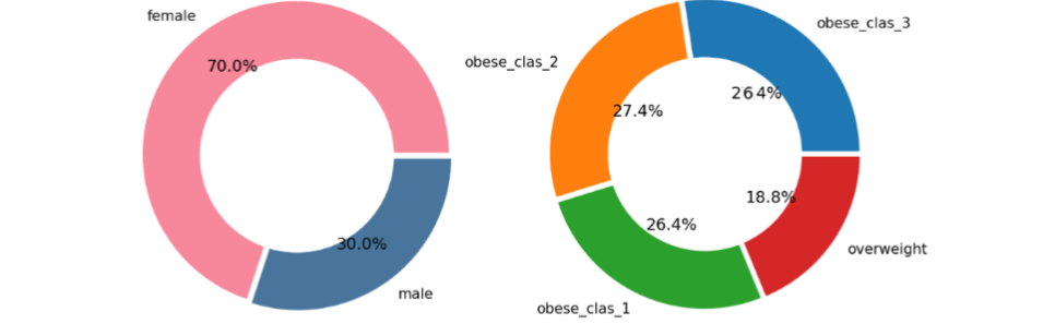
Figure 1 Total data
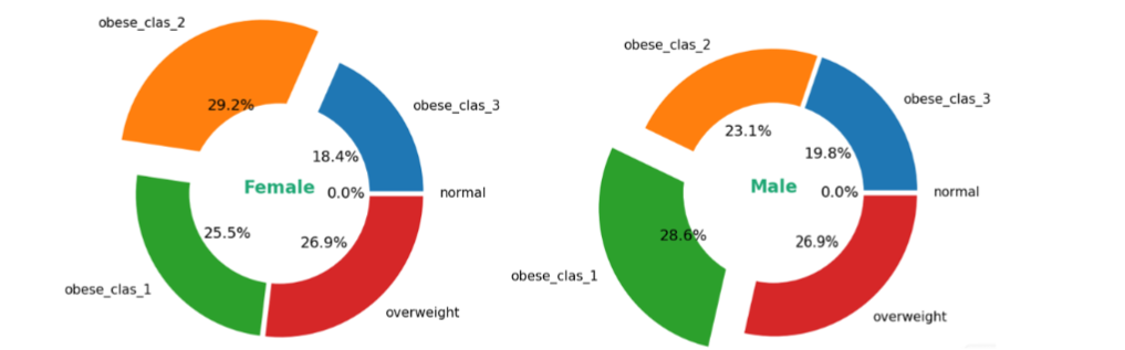
Figure 2 The Female and male comparison
In the Table 1 is presents the summary statistics of the clinical measurements used for calculations and analyses in this study. These statistics provide an overview of the central tendencies and dispersion of the variables, which include ALT (Alanine Aminotransferase), cholesterol, glucose, body mass, sex, systolic blood pressure (bp_s), and diastolic blood pressure (bp_d). This dataset serves as the foundation for all subsequent calculations and analyses conducted in this study. As it can be seen from table the lowest value of ALT is 10.0 and the highest value is 59.9. The average value of ALT is 29.846. The highest cholesterol is 8.1, the lowest value is 3.3 and the average is 5.7. The value of glucose is between 3.5 and 11.5. The average value of glucose is 5.358. The body mass is between 150.7 and 71 kg.
Table 1 Summary Statistics of Clinical Measurements for Patient Datase
| ALT | cholesterol | glucose | body_mass | sex | bp_s | bp_d | |
|---|---|---|---|---|---|---|---|
| count | 100 | 100 | 100 | 100 | 100 | 100 | 100 |
| mean | 29.845928 | 5.70 | 5.357655 | 110.35 | 0.296417 | 127.807818 | 84.283388 |
| std | 12.471018 | 1.041955 | 1.099450 | 19.902442 | 0.457423 | 23.013470 | 11.749335 |
| min | 10.000000 | 3.300000 | 3.500000 | 71.000000 | 0.000000 | 110.000000 | 70.000000 |
| max | 59.900000 | 8.100000 | 11.500000 | 150.700000 | 1.000000 | 290.000000 | 130.000000 |
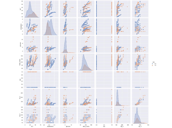
Figure 3 The scatterplot matrix of relationships between clinical variables, with points colored by sex.
The given plot (see Figure 3) is a pair plot (also known as a scatterplot matrix) that visualizes the relationships between several variables (ALT, cholesterol, glucose, diastolic blood pressure, systolic blood pressure), with points colored by sex.
STATISTICAL ANALYSIS OF THREE-FACTOR EXPERIMENTAL DESIGN
Patients were placed on a very low calorie diet with a daily intake of 750–900 calories minimum to 1200 maximum kcal, but reach with quality protein, distributed in short yet frequent meals (usually 5 meals per day) of functional food³⁴⁻³⁶. The protein food contains bioactive peptides and proteins and rich in vitamins and minerals³⁵, ³⁷⁻³⁸. They were closely observed by medical professionals working to treat their weight 8 visits for 4 months or over³⁹⁻⁴⁰.
The three-factor experimental design with two levels of variation (2^3 = 8) was used to assess the impact of these key parameters on body weight (Y). The main goal was to determine the relative importance of each of these factors on the response, which is weight reduction. The three parameters are considered: ALT enzyme (factor X1), total cholesterol (factor X2), and glucose (factor X3).
The three-factor experimental design⁴¹⁻⁴³ can be expressed in full (explicit representation) matrix form as follows:
also can be expressed in the shorter matrix form as:
y = Xb [2]
The regression model and analysis were performed using Python [44], employing regression equations, Cochran’s test, Student’s t-test, and Fisher’s test
For each series for each patient, a combination of factors for high and low levels has been made, along with measurements of the questionnaire and has two responses y₁ and y₂. y_av is an average of those responses. S²j is the variance of each response¹⁻²,⁴¹.
To determine that the order of dispersions is considered homogeneous, it is necessary to calculate Cochran’s criterion [45]. It is differences between three or more matched sets of frequencies or proportions. Using Cochran’s criterion, we are testing hypotheses for reproductive experiments⁴⁶⁻⁴⁹.
1. Cochran’s Test for Homogeneity:
To determine the homogeneity of variances, Cochran’s [3, 45, 50] criterion is given with formula:
Gp = max S²j / Σⱼ₌₁ᴺ S²j [3]
The critical value of Cochran’s test, Gα,f,N, is read from standard statistical tables corresponding to the 95% confidence interval, degrees of freedom, the number of experiments (N-8), and the number of levels of variation (k=2). The test statistic Gp is calculated from the observed data (see equation 2). If criteria Gp > Gα,f,N is satisfied then statistical heterogeneity is determined, but if Gp ≤ Gα,f,N, is presented then the order of variances of dispersions is considered as homogeneous [3].
2. Regression Model:
The linear three-factor model¹⁻²,⁵¹ is given by:
y = β₀ + β₁x₁ + β₂x₂ + β₃x₃ + β₁₂x₁x₂ + β₁₃x₁x₃ + β₂₃x₂x₃ + β₁₂₃x₁x₂x₃ [4]
where y is factor of stress, for the corresponding measurements yi1 and yi1, the factors xi, x₂, x₃, their units are given in the table 1, while βi represent coefficients of regression and βij coefficient of interaction between factors. Some coefficients may be negligibly small or insignificant. The determination of the significance of the regression coefficients is done with the help of the Student’s test criterion. In order to determine whether they are significant or not, first of all, the variance in which they are determined should be assessed:
3. Significance of Regression Coefficients:
Using the Student’s t-test [45]:
t = βi / Sβi [5]
Coefficients are significant if |βi| ≥ Sβi · t
4. Fisher’s Test for Model Adequacy:
The adequacy of the model was verified using Fisher’s criterion⁴⁰⁻⁴⁹:
Fp = S²ad / S²j = [Σⱼ₌₁ᴺ (yav − yi)² / (N − k − 1)] / S²j variance of adequacy / variance of each response [6]
Σⱼ₌₁ᴺ (yav − yi)² is the sum of the squared differences between the average response (yav) and the observed response (y). N is the number of experiments, k is the number of factors, N−k−1 is the degrees of freedom for the residual variance.
If the calculated F-ratio is less than the critical value from the F-distribution table, the model is considered adequate.
5. Transformation to Natural Units:
Conversion from coded variables to natural units was performed using:
xi = (Xi − X̄i) / ΔXi [7]
where: Xi – natural variable (factor), X̄i – average of coded variable, ΔXi – the interval of change of Xi (standard deviation), xi – coded variable [41].
Transformation to natural units is done to convert the coded variables used in the experimental design back to their original scale. Results in coded units can be difficult to interpret. Transforming them back to natural units makes it easier to understand the practical significance of the results. When applying the model to real-world scenarios or making predictions, it is necessary to use the natural units of the variables. This ensures that the predictions and conclusions are directly relevant to the actual conditions of the experiment.
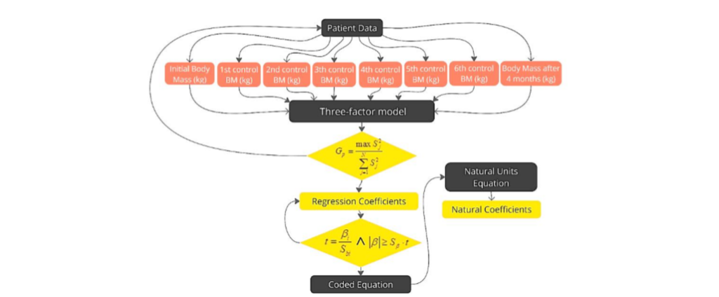
Figure 4 The Algorithm of traditional statistical three-factor model.
MACHINE LEARNING METHODS
In addition to the traditional statistical three-factor model, we utilized several ML algorithms to analyze the factors influencing obesity. These included Multiple Linear Regression, Decision Tree Regression, and Random Forest⁵²⁻⁵⁵. Each method was implemented to evaluate their effectiveness in identifying the key factors contributing to obesity.
DATA PREPROCESSING
Before applying ML models [55] the dataset was preprocessed as follows:
- Label Encoding: Categorical variables (such as category of obesity) were encoded into numerical values using label encoding.
- Cleaning data: Missing data can arise from various reasons such as data entry errors or participants missing appointments. It is essential to handle these missing values to maintain the integrity of the dataset.
After preprocessing data is splitted od training and testing set using the function “train_test_split”. Function splits the dataset into training (80%) and testing (20%) sets.
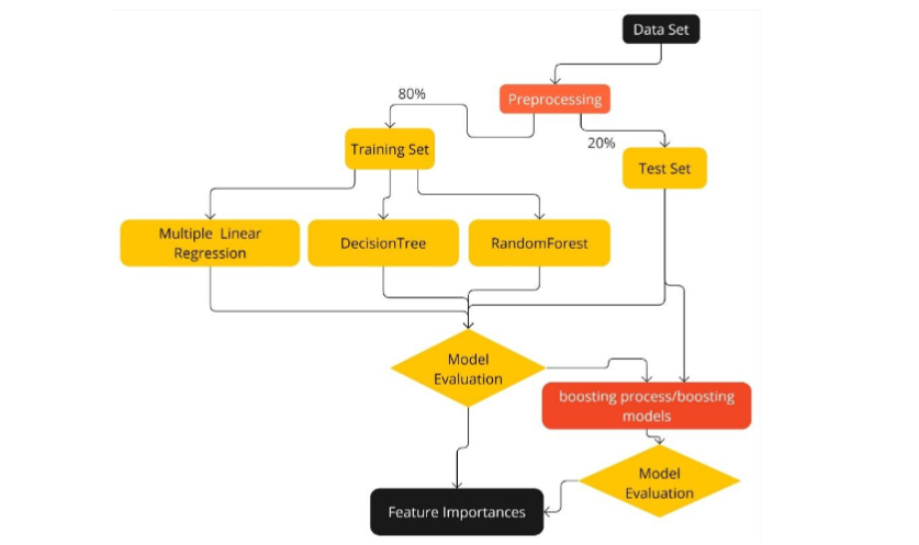
Figure 5 The Algorithm ML prediction in Python.
MODEL IMPLEMENTATION
Multiple Linear Regression
Dealing with Multiple Linear Regression [55, 44] includes several independent variables (x1, x2, …, xp), which the model is expressed as:
Y(yi) = β0 + β1×1 + β2×2 + … + βpxp [8]
the observed value is present with Y(yi)
To predict outcomes, the model is formulated as:
Y = β0 + β1X1 + β2X2 + … + βpXp + ε [9]
Y denotes the predicted value of the dependent variable Y based on given independent variables.
β0 is the y-intercept, indicating the expected value of Y when all independent variables are zero.
β1, β2, …, βp are the coefficients (slopes) for the respective independent variables.
ε (error or residual) is the discrepancy between the actual observed value (Y(yi)) and the predicted value (Ŷ), it is expressed as:
ε = yi − ŷi [10]
The main goal of linear regression is to find the coefficients that minimize the sum of squared errors (SSE) to provide a reliable model for predicting the target variable using the input features. This is typically achieved through techniques such as the least squares method, which optimizes the coefficients to develop a predictive model.
DECISION TREE REGRESSION
Decision trees are non-parametric models that split the data into subsets based on feature values, creating a tree-like structure of decisions. They are easy to interpret but prone to overfitting. A decision tree makes splits based on the feature that maximizes the information gain or minimizes the Gini impurity. For binary classification, the Gini impurity for a node with mmm samples is defined as [44, 56]:
G = 1 − Σᶜᵢ₌₁ (pi)² [11]
where pi is the proportion of samples belonging to class iii in the node and C is the number of classes. The information gain is the reduction in entropy after a split:
IG = H(X) − Σⁿᵢ₌₁ |Xi|/|X| H(Xi) [12]
where H(X) is the entropy of the parent node and H(X(i)) is the entropy of the i-th child node.
RANDOM FOREST REGRESSION
Random forests are an ensemble method that constructs multiple decision trees and averages their predictions. This reduces overfitting and improves generalization. A random forest constructs B decision trees on different bootstrap samples of the dataset and averages their predictions. The prediction for a sample is given by [44-56]:
y = 1/B Σᴮᵦ₌₁ hb(x) [13]
where hb(x) is the prediction of the b-th decision tree for input x.
The feature importance is calculated as the average decrease in Gini impurity (or increase in information gain) across all trees:
FIj = 1/B Σᴮᵦ₌₁ FIj,b [14]
where FIj,b is the importance of feature j in tree b.
GRADIENT BOOSTING REGRESSOR
It is a machine learning technique for regression problems. It builds an additive model in a forward stage-wise manner; each new tree attempts to correct errors made by the previously built ensemble [57]. The goal is to minimize the loss function L which measures the difference between the actual values yi and the predicted values ŷi:
∂L(φ) = Σⁿᵢ₌₁ l(yi, ŷi) [15]
Where yi is the actual value, ŷi is the predicted value, l is the loss function (e.g., mean squared error for regression).
For each data point i, the gradient of the loss function is:
gᵢ⁽ᵗ⁾ = ∂L(yi, ŷi⁽ᵗ⁻¹⁾) / ∂ŷi⁽ᵗ⁻¹⁾ [16]
Gradient descent:
The new tree gt is fit to the negative gradient of the loss function with respect to the current predictions:
rᵢ⁽ᵗ⁾ = − [∂L(yi, ŷi⁽ᵗ⁻¹⁾) / ∂ŷi⁽ᵗ⁻¹⁾] [17]
Where rᵢ⁽ᵗ⁾ are the residuals (errors) at iteration t
XGBOOST (EXTREME GRADIENT BOOSTING)
It is an implementation of gradient-boosted decision trees designed for speed and performance. The algorithm iteratively builds new trees that improve on the errors of the existing ensemble. The goal is to minimize the objective function L, which combines a loss function l that measures how well the model fits the data and a regularization term Ω that penalizes model complexity [Smola, A.]:
L(φ) = Σⁿᵢ₌₁ l(yi, ŷi) + Σᴷₖ₌₁ Ω(fk) [18]
Where, yi is the actual value, ŷi is the predicted value and Ω(fk) the is the regularization term for the k-th tree.
MODEL EVALUATION
The performance of the ML models was evaluated using metrics such as accuracy, R-squared (R²), Mean Squared Error (MSE), Root Mean Squared Error (RMSE): to compare their predictive power⁵²,⁵⁷.
Accuracy:
Measures the proportion of correctly predicted instances out of the total instances. It is generally used for classification problems.
Accuracy = Number of correct predictions / Total number of predictions [19]
R² Score:
Indicates the proportion of the variance in the dependent variable that is predictable from the independent variables. It ranges from 0 to 1, where 1 indicates perfect prediction [56-57].
R² Score:
R² = 1 − [Σ(yi − ŷ)² / Σ(yi − ȳ)²] [20]
R² Score: Reflects how well the model explains the variance in the data. Higher R² values indicate better explanatory power.
Mean Squared Error (MSE):
Measures the average of the squares of the errors, which is the average squared difference between the estimated values and the actual value.
MSE = 1/N Σⁿᵢ₌₁ (yi − ŷ)² [21]
Root Mean Squared Error (RMSE)
RMSE = √MSE = √[1/N Σⁿᵢ₌₁ (yi − ŷ)²] [22]
Root Mean Squared Error (RMSE): Is the square root of the mean of the squared errors. It provides a measure of the average magnitude of the errors in a set of predictions [56-57], predictions with lower RMSE values is more precise.
Results
In Table 2 is given a detailed overview of the parameters of anthropometric indicators BMI, and blood parameters according to gender after 8 controls.
Table 2 Summary of Control Parameters and Program Outcomes by Gender
| Parameters | female [min-max] ± SD | male [min-max] ± SD |
|---|---|---|
| Number of controls | [8] | [8] |
| Number of days of program | [40-210] ± 170 | [40-247] ± 155 |
| Desired body mass [kg] | [50-80] ± 8,2 | [74-90] ± 10,0 |
| Body mass after 4 month and over [kg] | [58-85] ± 9,1 | [75-98] ± 8,8 |
| The loss of weight [%] | [28-38] ± 3,0 | [24-36] ± 7,6 |
| After 4 month and over BMI [kg/m²] | [23,1-28,9 ± 3,8] | [24,0-32,2] ± 2,8 |
| ALT [U/L] (After 4 month and over) | 10-45 ± 18 | 10-40 ± 15 |
| Cholesterol [mol/L] (After 4 month and over) | 3-3,3 ± 1,3 | 3-3,5 ± 1,2 |
| Glucose [mol/L] (After 4 month and over) | 3-3,6 ± 1,2 | 3,3-3,6 ± 1,2 |
The data showcases the significant impact of the diet regime on various health parameters for both genders. Females showed a greater range of body mass reduction, while males exhibited consistent improvements in cholesterol and glucose levels. Overall, the diet effectively contributed to weight loss and improvement in key health markers over the monitored period.
To further understand the impact of the diet, a three-factorial design was employed using detailed patient data, including body mass (BM), for 8 controls (see Figure 4). This data is essential for calculating the Coded Equation (y) and the Natural Units Equation (Y). Table 3 summarizes all the regression equations in both coded and natural units along with relevant patient data for a better understanding of factors of influence of obesity. A preview calculation for 15 randomly chosen patients was conducted, but the model was applied to all 100 participants in the diet regime. This approach helps in understanding the interactions between variables such as body mass, BMI, and other health indicators, contributing to a comprehensive analysis of the diet’s effects. Key Findings: Glucose (X3) has the highest positive impact on body mass in both coded and natural unit equations. Cholesterol (X2) also has a significant positive impact on body mass. ALT (X1) has a smaller but still positive impact on body mass.
mass. The interaction between cholesterol and glucose (X23) is significant, indicating that the combined effect of these two factors is important in determining body mass⁵⁸.
These equations can be used to predict body mass based on ALT, cholesterol, and glucose levels. They can help in identifying which factors need to be controlled or monitored to manage body mass effectively. The natural units equation is particularly useful for healthcare professionals and researchers for making real-world predictions and interventions. Visualizations help to identify how well the model captures the influence of ALT, cholesterol, and glucose on body mass, highlighting any discrepancies between the actual and predicted data. Figure 6 presents the actual and predicted body mass values alongside ALT, cholesterol, and glucose levels. The three plots illustrate the relationships between these factors and body mass, comparing the real measurements with the predicted values from a regression model.
Table 3 Comparison of Actual and Predicted Body Mass with ALT, Cholesterol, and Glucose Levels
| No | sex | age | Initial BM (kg) | BM after 4 months (kg) | Height (m) | Initial BMI (kg/m²) | BMI after 4 months (kg/m²) | Coded Equation (y) and Natural Units Equation (Y) |
|---|---|---|---|---|---|---|---|---|
| 1 | m | 55 | 149,5 | 82,5 | 186 | 43,2 | 24.0 | y = 107.25 + 4.412x₁ + 8.312x₂ + 18.288x₃ + 3.7x₂₃ / Y = 1.29 + 0.25X₁ + 6.65X₂ + 15.9X₃ + 2.4X₂₃ |
| 2 | m | 37 | 116 | 92 | 169 | 40,6 | 32,2 | y = 97,2875 + 3,8875x₂ + 5,3375x₃ + 2,8375x₂₃ / Y = 80,7476 − 5,67385X₂ + 3,7377X₃ + 1,9739X₂₃ |
| 3 | f | 34 | 90 | 75 | 158 | 36,1 | 30,0 | y = 79.1125 + 2.5625x₂ + 3.7125x₃ / Y = 56.03 + 2.05X₂ + 3.23X₃ |
| 4 | f | 65 | 107 | 75 | 163 | 40,3 | 28,2 | y = 85.65 + 2.19x₁ + 4.64x₂ + 7.78x₃ / Y = 66.16 + 0.13X₁ + 3.715X₂ + 6.77X₃ |
| 5 | f | 33 | 130,8 | 76,2 | 164 | 48,6 | 28,3 | y = 103.212 + 6.54x₂ + 10.9x₃ / Y = 38.81 + 5.23X₂ + 9.48X₃ |
| 6 | f | 36 | 133,3 | 75 | 181 | 40,7 | 23.0 | y = 99.93 + 2.89x₁ + 4.99x₂ + 18x₃ / Y = 59.93 + 0.17X₁ + 3.99X₂ + 16.29X₃ |
| 7 | f | 44 | 161,6 | 85 | 170 | 55,9 | 29,4 | y = 128.75 + 4.26x₁ + 7.65x₂ + 12.5x₃ / Y = 47.31 + 0.24X₁ + 6.1X₂ + 10.95X₃ |
| 8 | m | 42 | 135 | 93 | 180 | 41,7 | 28,7 | y = 103.75 + 4.26x₁ + 7.65x₂ + 12.5x₃ / Y = 73.53 + 0.20X₁ + 5X₂ + 9.04X₃ |
| 9 | m | 48 | 123,7 | 96 | 170 | 39,9 | 31,0 | y = 101.175 + 4.2x₂ + 4.85x₃ / Y = 59.49 + 3.38Y₂ + 4.22Y₃ |
| 10 | m | 42 | 129,6 | 75,9 | 176 | 41,8 | 24,5 | y = 98.31 + 3.8x₁ + 6.8x₂ + 15.06x₃ / Y = 10.87 + 0.22X₁ + 5.45X₂ + 13.10X₃ |
| 11 | m | 62 | 121,2 | 90 | 172 | 41,0 | 30,4 | y = 96.575 + 8.075x₃ / Y = 65.33 + 7.02X₃ |
| 12 | m | 39 | 144,7 | 95 | 181 | 44,2 | 29,0 | y = 112.48 + 6.23x₂ + 11.48x₃ / Y = 46.87 + 4.99X₂ + 9.98X₃ |
| 13 | m | 45 | 104,6 | 79 | 168 | 37,1 | 28,0 | y = 87.48 + 1.9x₁ + 3.05x₂ + 6.36x₃ / Y = 49.49 + 0.11X₁ + 2.44X₂ + 5.53X₃ |
| 99 | f | 43 | 98,8 | 60 | 154,4 | 41,4 | 25,2 | y = 85.91 + 2x₁ + 4.1x₂ + 9.8x₃ / Y = 30.63 + 0.12X₁ + 3.28X₂ + 8.55X₃ |
| 100 | f | 51 | 120 | 70 | 159 | 47,5 | 27,7 | y = 89 + 4.5x₁ + 7.35x₂ + 11.38x₃ / Y = 13.73 + 0.24X₁ + 5.9X₂ + 9.89X₃ |
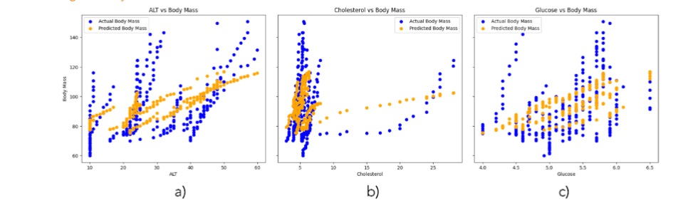
Figure 6 Comparison of Actual and Predicted Body Mass with ALT, Cholesterol, and Glucose Levels
The three plots (see Figure 6) illustrate the relationship between different factors (ALT, cholesterol, and glucose) and body mass, comparing the actual body mass measurements with the predicted values from a regression model. The distribution of blue dots (actual measurements) indicates how body mass varies with ALT, cholesterol, and glucose levels. The orange dots (predicted values) should ideally align closely with the blue dots if the model predicts well.
a) In this plot, there is a visible clustering of actual and predicted values around certain ALT levels, suggesting some correlation. However, there is also a noticeable spread, indicating variability in body mass that the model might not fully capture.
b) This plot suggests a clearer relationship between cholesterol and body mass, with the predicted values aligning more closely with the actual values, indicating that cholesterol might be a significant predictor of body mass in this model.
c) This plot suggests a significant correlation between glucose levels and body mass, with predicted values aligning well with actual values, indicating that glucose is an important predictor of body mass.
While the three-factor experimental design focused primarily on glucose, ALT enzyme, and cholesterol, the machine-learning models expanded the analysis to include additional factors such as body mass, blood pressure, and sex. This combined approach allowed for a more nuanced understanding of how these variables interact and influence obesity, providing deeper insights into their relative impacts.
To enhance the robustness of our analysis, we incorporated Multiple Linear Regression, which included additional variables such as body mass, blood pressure, and sex. Mathematically, this approach is similar to the three-factorial design, allowing us to expand the model to include more variables while preserving the ability to analyze interactions between factors. During machine learning, for the given model (see Table 4), the metric parameters were obtained for checking the accuracy of the models. The accuracy of Multiple Linear Regression is 0.90, but MSE=4.526 and RMSE=2.128. Multiple Linear Regression performs well with high accuracy and moderate error rates. “Moderate error metrics” refers to the level of difference between the actual values and the predicted values by the model. A lower MSE indicates that the predictions are closer to the actual values. Here, the MSE is 4.526270, which suggests that while the model makes reasonably accurate predictions, there is still some room for improvement compared to the models with lower MSE. An RMSE of 2.127503 means that, on average, the predictions are about 2.13 units away from the actual values. This is considered moderate because it indicates that the predictions are fairly close to the actual values, but not as precise as those from the best-performing models in the comparison.
Decision Trees and Random Forest operate similarly in terms of decision-making methodology.
The decision tree model (see Figure 7) provides a visual representation of how different factors influence obesity categories. The root node starts with the body mass (BMI ≤ 91.4. This initial split helps distinguish between different obesity classes. First Level- Left Split: If the glucose level is ≤ 4.95, the model further examines body mass to categorize patients as overweight or class 1 obese. This branch highlights glucose as a significant factor in determining obesity levels. Right Split: For those with body mass ≤ 120.3, the model looks at ALT levels and sex, showing these factors’ importance in differentiating between class 2 and class 3 obesity. Second Level – Left Branch: Further divided by body mass, highlighting its role in distinguishing between overweight and class 1 obesity. Right Branch: Analyzes ALT levels and sex, indicating their combined effect on obesity categorization. Third Level -Cholesterol: The model examines cholesterol levels, further refining the classification into obesity classes. This indicates that cholesterol, while influential, plays a more nuanced role compared to other factors.
The decision tree (see Figure 7) clearly demonstrates how glucose, ALT, body mass, blood pressure, and sex contribute to predicting obesity categories. It visualizes the complex interactions between these factors, emphasizing the importance of a comprehensive approach to understanding obesity.
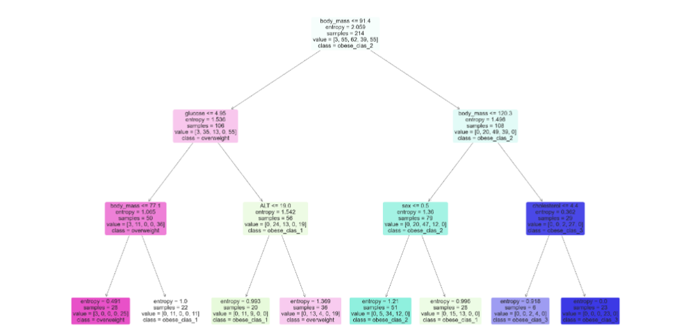
Figure 7 Decision Tree Visualization of Factors Influencing Obesity
The Decision Tree, with an accuracy of 0.81, MSE of 9.133, and RMSE of 3.022, shows lower accuracy and higher errors, suggesting less robustness. In contrast, the Random Forest model achieves better performance with an accuracy of 0.86, MSE of 6.898012, and RMSE of 2.626407, demonstrating a better balance of accuracy and error metrics. To further improve prediction results, boosting models like Gradient Boosting Regressor and XGBoost are employed. These models act as a boosting process to reduce overfitting and enhance prediction accuracy. As was expected Gradient Boosting Regressor and XGBoost models have the highest accuracy and the lowest errors, demonstrating superior predictive capabilities. This results are making them the most reliable for predicting the outcomes in this study.
Table 4 presents a comparison of model performance for both basic and boosting models.
Table 4 Model Performance Comparison
| Model | Training Accuracy | Testing Accuracy | R-squared | MSE | (RMSE) |
|---|---|---|---|---|---|
| Multiple Linear Regression | 0.910977 | 0.902875 | 0.902875 | 4.526270 | 2.127503 |
| Decision Tree | 0.88 | 0.81 | 0.810075 | 9.133131 | 3.022107 |
| Random Forest | 0.91 | 0.86 | 0.856555 | 6.898012 | 2.626407 |
| Gradient Boosting Regressor | 0.99 | 0.95 | 0.949479 | 2.429442 | 1.558667 |
| XGBoost | 0.99 | 0.95 | 0.954510 | 2.187526 | 1.479029 |
From the conducted feature importance analysis of the given ML models, the results are summarized in Table 5. It can be observed that body mass is the most significant factor influencing obesity, which aligns with general knowledge. However, machine learning models have confirmed that glucose is the next most significant factor, followed by cholesterol, ALT, and blood pressure. This analysis provides a comprehensive understanding of the relative importance of various factors affecting obesity, with body mass being the predominant factor, but also highlighting the significant roles of glucose and cholesterol.
Table 5 Feature importance
| feature importance | |
|---|---|
| 3 | body_mass |
| 2 | glucose |
| 1 | cholesterol |
| 0 | ALT |
| 5 | bp_s |
| 6 | bp_d |
| 4 | sex |
Discussion
This study contributes by integrating traditional statistical approaches, such as factorial design, with advanced machine learning models to analyze obesity factors and predict outcomes.
Traditional statistical methods, particularly the factorial design used in this study, have proven effective in identifying key variables like glucose, cholesterol, and ALT, as well as the influence of combining these factors. However, the main strength of our approach is demonstrating how well machine learning models can enhance prediction accuracy and offer a more comprehensive understanding of the data.
This finding is consistent with existing research, such as that presented by Thamrin et al.⁵⁹ and By Ferdowsy et al.⁶⁰, which also identify glucose levels as a major predictor of obesity in sugary foods, alcoholic drinks consumption, sweet drinks, fatty/oily foods, and soft/carbonated drinks.
Cholesterol (X2) was also found to have a substantial impact, albeit slightly less than glucose. This is in agreement with the findings of Chatterjee et al.⁶¹, who note that physiological factors like cholesterol, significantly contribute to obesity and cardiovascular disease.
The smaller but noticeable impact of ALT (X1) on obesity especially to female attendance in this study. Aligns with the literature, particularly DeGregory et al.⁶², who in the study apply neural networks, and deep learning and were evaluated using area under the curve for predicting high blood pressure and high body fat. But also is many studies that ALT is in relation with blood pressure⁵⁸.
The primary contribution of the machine learning analysis is not merely to reconfirm the influence of well-known factors like glucose and cholesterol but to rigorously assess how accurately these factors can predict obesity outcomes when modeled through advanced techniques³¹,⁶³. The decision tree model, for instance, not only provides a hierarchical understanding of obesity determinants but also showcases how machine learning can visualize and simplify decision-making processes. In this study, machine learning models, including Gradient Boosting Regressor and XGBoost, achieved the highest prediction accuracy (95%) and low RMSE values, significantly outperforming traditional regression models and results from other references for regression methods.
Conclusion
Integrating statistical methods with ML models provided a more comprehensive understanding of the factors affecting obesity, offering deeper insights into their relative impacts and interactions. This combined approach not only confirmed known predictors of obesity but also revealed the importance of considering multiple health parameters and the influence of combining these factors for accurate prediction and effective intervention.
Future research should continue to explore how combining these methodologies can provide even more precise and actionable insights into obesity management and intervention strategies.
Conflict of Interest:
None.
Funding Statement:
None.
Acknowledgements:
None.
References
1. Antony, J. (2014). Design of Experiments for Engineers and Scientists. Elsevier Ltd., 63-85.
2. NIST SEMATECH. e-Handbook of Statistical Methods. https://doi.org/10.18434/M32189.
3. Levine, M. D., Stephan, F. D. (2022). Even You Can Learn Statistics and Analytics: An Easy to Understand Guide to Statistics and Analytics (4th ed.). Pearson FT Press, 211-248.
4. Salsburg, D. (2002). The Lady Tasting Tea: How Statistics Revolutionized Science in the Twentieth Century. Henry Holt and Company. ISBN 0-8050-7134-2.
5. Jiju, A. (2014). Design of Experiments for Engineers and Scientists (2nd ed.). Elsevier, Amsterdam, Netherlands.
6. Das, K. A., Dewanjee, S. (2018). Optimisation of Extraction Using Mathematical Models and Computation. In: Sarker, D. S., Nahar, L. (Eds.), Computational Phytochemistry. Elsevier, Amsterdam, Netherlands, 75-106.
7. Ait-Amir, B., El Hami, A., Pougnet, P. (2020). Meta-Model Development. In: El Hami, A., Pougnet, P. (Eds.), Embedded Mechatronic Systems 2 (2nd ed.). Elsevier, Amsterdam, Netherlands. https://doi.org/10.1016/B978-1-78548-014-0.50006-2. Accessed 19 December 2022.
8. Antoska Knights, V., & Millaku, J. (2023). Three-factor experimental design as a tool in applied statistics. International Journal of Statistics and Applied Mathematics, 8(1), 46-49. https://doi.org/10.22271/maths.2023.v8.i1a.929
9. Markovikj, G., & Knights, V. (2022). Model of optimization of the sustainable diet indicators. Journal of Hygienic Engineering and Design, 39, 169-175.
10. Sun, Y., Wang, X., Zhang, C., & Zuo, M. (2023). Multiple Regression: Methodology and Applications. Highlights in Science, Engineering and Technology AMMSAC, 49, 542.
11. Gelman, A., & Hill, J. (2006). Data Analysis Using Regression and Multilevel/Hierarchical Models. Cambridge University Press.
12. Iwasaki, M. (2020). Multiple Regression Analysis from Data Science Perspective. In: Multiple Regression Analysis, 131-140. https://doi.org/10.1007/978-981-15-2700-5_8.
13. Kutner, M. H., Nachtsheim, C. J., Neter, J., & Li, W. (2004). Applied Linear Statistical Models. McGraw-Hill Education.
14. Knights, V., & Prchkovska, M. (2024). From equations to predictions: Understanding the mathematics and machine learning of multiple linear regression. Journal of Mathematical & Computer Applications, 3(2), 1-8. https://doi.org/10.47363/JMCA/2024(3)137
15. Cui, T., Chen, Y., Wang, J., Deng, H., & Huang, Y. (2021). Estimation of Obesity Levels Based on Decision Trees. 2021 International Symposium on Artificial Intelligence and its Application on Media (ISAIAM), 160-165. https://doi.org/10.1109/ISAIAM53259.2021.00041
16. Iparraguirre-Villanueva, O., Mirano-Portilla, L., Gamarra-Mendoza, M., & Robles-Espiritu, W. (2024). Predicting obesity in nutritional patients using decision tree modeling. International Journal of Advanced Computer Science and Applications. Retrieved from https://api.semanticscholar.org/CorpusID:268819010
17. Cui, T., Chen, Y., Wang, J., Deng, H., & Huang, Y. (2021). Estimation of obesity levels based on decision trees. In 2021 International Symposium on Artificial Intelligence and its Application on Media (ISAIAM) (pp. 160-165). Retrieved from https://api.semanticscholar.org/CorpusID:237296330
18. Rodríguez-Pardo, C., Segura, A., Zamorano-León, J. J., Martínez-Santos, C., Martínez, D., Collado-Yurrita, L., … & López-Farre, A. (2019). Decision tree learning to predict overweight/ obesity based on body mass index and gene polymorphisms. Gene, 699, 88-93. https://doi.org/10.1016/j.gene.2019.03.011
19. Han, S., Williamson, B. D., & Fong, Y. (2021). Improving random forest predictions in small datasets from two-phase sampling designs. BMC Medical Informatics and Decision Making, 21, 322. https://doi.org/10.1186/s12911-021-01688-3
20. Fernández-Delgado, M., Cernadas, E., Barro, S., & Amorim, D. (2014). Do we need hundreds of classifiers to solve real-world classification problems? Journal of Machine Learning Research, 15, 3133-3181.
21. Lu, X., & Bengio, Y. (2005). An analysis of the random subspace method for decision forest. In Proceedings of the 22nd International Conference on Machine Learning (ICML) (Vol. 1, pp. 497-504). New York, NY, USA.
22. Liaw, A., & Wiener, M. (2002). Classification and regression by random forest. R News, 2(3), 18-22.
23. Jana, M. (2023). Exploring Machine Learning Models: A Comprehensive Comparison of Logistic Regression, Decision Trees, SVM, Random Forest, and XGBoost. Medium. Available from: https://medium.com/@malli.learnings/exploring-machine-learning-models-a-comprehensive-comparison-of-logistic-regression-decision-38cc12287055
24. Lee, H., Wang, J., & Leblon, B. (2020). Using Linear Regression, Random Forests, and Support Vector Machine with Unmanned Aerial Vehicle Multispectral Images to Predict Canopy Nitrogen Weight in Corn. Remote Sensing, 12(13), 2071. https://doi.org/10.3390/rs12132071
25. Miotto, R., Wang, F., Wang, S., Jiang, X., & Dudley, J. T. (2018). Deep learning for healthcare: review, opportunities and challenges. Briefings in Bioinformatics, 19(6), 1236-1246. https://doi.org/10.1093/bib/bbx044
26. Maharana, A., & Nsoesie, E. O. (2018). Use of deep learning to examine the association of the built environment with prevalence of neighborhood adult obesity. JAMA Network Open, 1(4), e181535. https://doi.org/10.1001/jamanetworkopen.2018.1535
27. U, S., K. PT, & K, S. (2021). Computer aided diagnosis of obesity based on thermal imaging using various convolutional neural networks. Biomedical Signal Processing and Control, 63, 102233. https://doi.org/10.1016/j.bspc.2020.102233
28. James, G., Witten, D., Hastie, T., & Tibshirani, R. (2013). An Introduction to Statistical Learning. Springer.
29. Hastie, T., Tibshirani, R., & Friedman, J. (2001). The Elements of Statistical Learning: Data Mining, Inference, and Prediction. Springer.
30. Murphy, K. P. (2012). Machine Learning: A Probabilistic Perspective. MIT Press.
31. Knights, V., Kolak, M., Markovikj, G., & Gajdoš Kljusurić, J. (2023). Modeling and optimization with artificial intelligence in nutrition. Applied Sciences, 13(13), 7835.
32. Knights, V., Gavriloska, E. D., et al. (2024). Machine Learning Techniques for Modelling and Predicting the Influence of Kefir in a Low-Protein Diet on Kidney Function. Medical Research Archives, 12(7). https://doi.org/10.18103/mra.v12i7.0000
33. An, R., Shen, J., & Xiao, Y. (2022). Applications of Artificial Intelligence to Obesity Research: Scoping Review of Methodologies. Journal of Medical Internet Research, 24, e40589. https://doi.org/10.2196/40589
34. Markovikj, G., Knights, V., & Kljusurić, J. G. (2023). Ketogenic Diet Applied in Weight Reduction of Overweight and Obese Individuals with Progress Prediction by Use of the Modified Wishnofsky Equation. Nutrients, 15, 927. https://doi.org/10.3390/nu15040927
35. Markovikj, G., Knights, V., & Gajdoš Kljusurić, J. (2023). Body Weight Loss Efficiency in Overweight and Obese Adults in the Ketogenic Reduction Diet Program—Case Study. Applied Sciences, 13, 10704. https://doi.org/10.3390/app131910704
36. Markovikj, G., Knights, V., Nikolovska Nedelkovska, D., & Damjanovski, D. (2020). Statistical analysis of results in patients applying the sustainable diet indicators. Journal of Hygienic Engineering and Design, 30, 35–39. https://doi.org/10.3390/app131910704
37. Westman, E. (2013). A Low Carbohydrate, Ketogenic Diet Manual: No Sugar, No Starch Diet. CreateSpace Independent Publishing Platform, Scotts Valley, USA.
38. Moore, J., & Westman, C. M. D. (2014). Keto Clarity. Retrieved from https://www.scribd.com/document/412124479/Keto-Clarity-by-Jimmy-Moore-and-Eric-Westman-MD. Accessed 8 December 2022.
39. Greene, W. H. (2018). Econometric Analysis. Pearson Education. Available at: https://www.ctanujit.org/uploads/2/5/3/9/25393293/_econometric_analysis_by_greence.pdf
40. Hastie, T., Tibshirani, R., & Friedman, J. (2009). The Elements of Statistical Learning. Springer.
41. Montgomery, D. C. (2013). Design and Analysis of Experiments (8th ed.). John Wiley & Sons.
42. Anderson, M., & Whitcomb, P. (2007). DOE Simplified: Practical Tools for Effective Experimentation (2nd ed.). Retrieved from https://cdnm.statease.com/pubs/doesimp2excerpt–chap3.pdf
43. IMCF Designs. (2013). Experimental Design: Multiple Independent Variables. Retrieved from https://uca.edu/psychology/files/2013/08/Ch13-Experimental-Design_Multiple-Independent-Variables.pdf
44. Müller, A. C., & Guido, S. (2016). Introduction to Machine Learning with Python: A Guide for Data Scientists. O’Reilly Media. Available at https://www.nrigroupindia.com/e-book/Introduction%20to%20Machine%20Learning%20with%20Python%20(%20PDFDrive.com%20)-min.pdf
45. Sheskin, D. J. (2000). Handbook of Parametric and Nonparametric Statistical Procedures (2nd ed.). Chapman & Hall/CRC.
46. Kiemele, M. J., Schmidt, S. R., & Berdine, R. J. (1997). Basic Statistics: Tools for Continuous Improvement (4th ed.). Air Academy Press.
47. James, G., Witten, D., Hastie, T., & Tibshirani, R. (2013). An Introduction to Statistical Learning: With Applications in R. Springer.
48. Dean, A., Morris, M., Stufken, J., & Bingham, D. (Eds.). (2015). Handbook of Design and Analysis of Experiments. CRC Press.
49. Dean, A. M., & Voss, D. T. (1999). Design and Analysis of Experiments. Springer.
50. Lane, D. M., Scott, D., Hebl, M., Guerra, R., Osherson, D., & Zimmer, H. (2024). Introduction to Statistics (Online ed.). Rice University; University of Houston, Downtown Campus. Available at: Online _Statistics_Education.pdf (onlinestatbook.com)
51. Leonardo, A. (2024). The Practically Cheating Statistics Handbook (5th ed.). Practically Cheating. Available at: Tables – Statistics How To
52. Thakur, A. (2020). Approaching (Almost) Any Machine Learning Problem. Independently published.
53. Burkov, A. (2019). The Hundred-Page Machine Learning Book. Andriy Burkov.
54. Boehmke, B., & Greenwell, B. (2019). Hands-On Machine Learning with R. CRC Press.
55. Deisenroth, M. P., Faisal, A. A., & Ong, C. S. (2020). Mathematics for Machine Learning. Cambridge University Press. https://mml-book.com
56. Smola, A., & Vishwanathan, S. V. N. (2008). Introduction to Machine Learning. Cambridge University Press. Available at https://alex.smola.org/drafts/thebook.pdf
57. Mitchell, T. M. (1997). Machine Learning. McGraw-Hill Science/Engineering/Math. Available at https://www.cin.ufpe.br/~cavmj/Machine%20-%20Learning%20-%20Tom%20Mitchell.pdf
58. Yao, X., Hu, K., & Wang, Z. et al. (2024). Liver indicators affecting the relationship between BMI and hypertension in type 2 diabetes: a mediation analysis. Diabetology & Metabolic Syndrome, 16, 19. https://doi.org/10.1186/s13098-023-01254-z
59. Thamrin, Sri Astuti, Dian Sidik Arsyad, Hedi Kuswanto, Armin Lawi, and Sudirman Nasir. “Predicting Obesity in Adults Using Machine Learning Techniques: An Analysis of Indonesian Basic Health Research 2018.” Frontiers in Nutrition 8 (2021): Article 669155. https://doi.org/10.3389/fnut.2021.669155
60. Ferdowsy, Faria, Kazi Samsul Alam Rahi, Md. Ismail Jabiullah, and Md. Tarek Habib. “A Machine Learning Approach for Obesity Risk Prediction.” Current Research in Behavioral Sciences 2 (2021): 100053. https://doi.org/10.1016/j.crbeha.2021.100053
61. Chatterjee, Ayan, Martin W. Gerdes, and Santiago G. Martinez. “Identification of Risk Factors Associated with Obesity and Overweight—A Machine Learning Overview.” Sensors 20, no. 9 (2020): 2734. https://doi.org/10.3390/s20092734
62. DeGregory, K. W., P. Kuiper, T. DeSilvio, J. D. Pleuss, R. Miller, J. W. Roginski, C. B. Fisher, D. Harness, S. Viswanath, S. B. Heymsfield, I. Dungan, and D. M. Thomas. “A Review of Machine Learning in Obesity.” Obesity Reviews: An Official Journal of the International Association for the Study of Obesity 19, no. 5 (2018): 668-685. Safaei, Mahmood, Elankovan A. Sundararajan, Maha Driss, Wadii Boulila, and Azrulhizam Shapi’i. “A Systematic Literature Review on Obesity: Understanding the Causes & Consequences of Obesity and Reviewing Various Machine Learning Approaches Used to Predict Obesity.” Computers in Biology and Medicine 136 (2021): 104754. https://doi.org/10.1016/j.compbiomed.2021.104754
63. https://doi.org/10.1111/obr.12667