Bioelectrical Impedance Analysis for Breast Cancer: Diagnosis, Prognosis, and Tissue Mapping

Donato M. Ceres, PhD,¹ Wendy M. Mikkelson, MD,² Christopher W. Gregory, PhD,³ James J. Marx, PhD,⁴ William D. Gregory, PhD⁵

1. Chief Science Officer, NovaScan Inc., Chicago, IL, USA
2. Director, Advocate Aurora St. Luke’s Comprehensive Breast Health Center, Milwaukee, WI, USA (retired)
3. Lane Department of Computer Science and Electrical Engineering, West Virginia University, Morgantown, WV, USA
4. Advocate Aurora Health Care, Milwaukee, WI, USA (retired)
5. Professor Emeritus, Department of Electrical Engineering, and College of Health Professions & Sciences, University of Wisconsin, Milwaukee, WI, USA

OPEN ACCESS

PUBLISHED: 31 May 2025

CITATION: Ceres, D. M., 2025. Bioelectrical Impedance Analysis for Breast Cancer: Diagnosis, Prognosis, and Tissue Mapping. Medical Research Archives, [online] 13(5).
https://doi.org/10.18103/mra.v13i5.6306

COPYRIGHT: © 2025 European Society of Medicine. This is an open-access article distributed under the terms of the Creative Commons Attribution License, which permits unrestricted use, distribution, and reproduction in any medium, provided the original author and source are credited.

DOI https://doi.org/10.18103/mra.v13i5.6306

ISSN 2375-1924

ABSTRACT

Breast cancer remains one of the most diagnosed malignancies, necessitating early detection and accurate prognostic assessment. Traditional imaging methods play a crucial role in screening but often lack specificity, particularly in patients with dense breast tissue. Histopathological examination is still the gold standard but is invasive and time-consuming.

Bioelectrical impedance analysis is a promising non-invasive method for detecting malignancies by examining tissue electrical properties. The Cole relaxation frequency (CRF), derived from impedance spectroscopy, effectively differentiates malignant from benign breast tissue and serves as a strong prognostic marker. Elevated CRF values correlate with changes in cellular structure and membrane polarization, helping to predict recurrence risk and metastatic potential.

Electrical Property Enhanced Tomography represents a significant advancement over traditional electrical impedance-based imaging techniques by integrating external anatomical imaging modalities to enhance spatial resolution. This method uses anatomical data to guide impedance-based reconstructions, thereby effectively reducing the error and instability commonly associated with conventional approaches. As a result, the accuracy of tissue property mapping is substantially improved. In addition, the structured placement of electrodes, combined with the application of a conductive bolus, contributes to greater measurement consistency and reliability.

Beyond breast cancer, intraoperative CRF and other impedance-derived features, combined with AI-driven machine learning algorithms, have shown promise for surgical margin assessment in dermal tissues, improving precision and workflow efficiency. This review summarizes more than two decades of the authors’ work on the use of bioelectrical impedance in cancer research and clinical applications.

Introduction

Breast cancer remains the most frequently diagnosed cancer among women worldwide and a leading cause of cancer-related mortality.¹ Early and accurate detection is essential to improving patient outcomes,² as localized breast cancer is often highly treatable,³ whereas metastatic disease significantly reduces survival rates.⁴⁻⁷ Traditional diagnostic methods such as mammography, ultrasound, and magnetic resonance imaging (MRI) are widely used for early detection, yet they have inherent limitations, including difficulties in differentiating between benign and malignant lesions,⁸˒⁹ as well as reduced sensitivity in patients with dense breast tissue.¹⁰ While histopathology remains the gold standard for definitive cancer diagnosis, it is an invasive and time-consuming process that introduces delays¹¹ in treatment planning and is associated with patient discomfort and risk of complications.¹²

Given these challenges, there is a growing interest in developing alternative, non-invasive, and real-time diagnostic methods that can accurately distinguish cancer from healthy tissue. One such promising approach is bioelectrical impedance analysis, which measures the electrical properties of biological tissues to detect pathological changes at the cellular level.¹⁴˒¹⁵ Within this field, the Cole relaxation frequency (CRF) has emerged as a particularly effective diagnostic indicator for breast cancer.¹⁶ This parameter, derived from the spectral impedance, reflects the electrical response of tissues across different frequencies and has been shown to be highly sensitive to malignancy.¹⁷ CRF not only enables accurate differentiation between benign and malignant breast tissue but also holds prognostic value by predicting the likelihood of recurrence and metastasis following surgical excision.¹⁸

Over the past two decades, the authors have investigated multiple bioelectrical impedance features across a range of human tissues, beginning with the breast and subsequently extending to the lung,¹⁹ skin,¹⁸ pancreas,²⁰ and gastrointestinal tract. These efforts have encompassed the use of impedance spectroscopy to analyze excised tissues for diagnostic purposes, as well as long-term prognostic studies validated through retrospective follow-up after ten years.²¹ In addition to single-point measurements,¹⁶ methods have been developed to generate spatially resolved impedance maps, enabling both microscopic assessment of tumor margins in excised specimens and macroscopic imaging of disease distribution across the entire breast.²²

This review also presents a new mathematical framework designed to improve in-vivo imaging of tissue electrical properties to maximize accuracy and spatial resolution. We conclude with a discussion on how these impedance-based methodologies can be integrated into the clinical workflow, spanning screening, diagnosis, treatment, and long-term follow-up.

---

Connecting Electrical Impedance and Cell Biology

Bioelectrical impedance is a fundamental property of biological tissues that depends on the ability of cells to conduct and store electrical charge.²³˒²⁴ It varies across different tissue types due to differences in cellular structure, membrane composition, and extracellular matrix organization.²⁵˒²⁶ The conductivity and permittivity of tissues influence their impedance behavior,²⁷ with cancerous tissues displaying significantly altered electrical properties due to increased cellular density,²⁸ disorganized architecture,²⁹ and enhanced metabolic activity.³⁰ These alterations affect the flow of ionic current and result in distinct impedance spectra when compared to normal or benign tissues.³¹˒³²

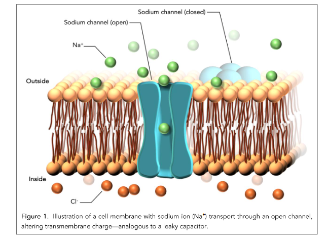
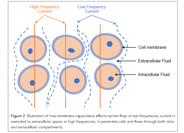
Figure 1 illustrates a biological lipid bilayer with an embedded ion channel, highlighting a fundamental component of cellular electrical properties measured in bioelectrical impedance spectroscopy (BIS). In the context of cancer detection, BIS exploits differences in how electrical currents interact with tissues, particularly how they traverse cell membranes and their associated ion channels.³³˒³⁴ The lipid bilayer serves as an insulating barrier,³⁵ while ion channels allow selective ionic movement,³⁶˒³⁷ contributing to the capacitive and resistive characteristics of the tissue.³⁸ Cancerous tissue often exhibits altered membrane composition,³⁹ ion channel expression,⁴⁰ and cellular architecture, which in turn affect impedance spectra across a range of frequencies. At lower frequencies, current tends to flow around intact cells, reflecting extracellular resistance, whereas at higher frequencies, it can penetrate membranes, revealing intracellular properties (Figure 2).⁴¹˒⁴² Therefore, changes in the structure and function of membranes and ion channels are central to the electrical signatures that BIS uses to distinguish healthy from malignant tissue.

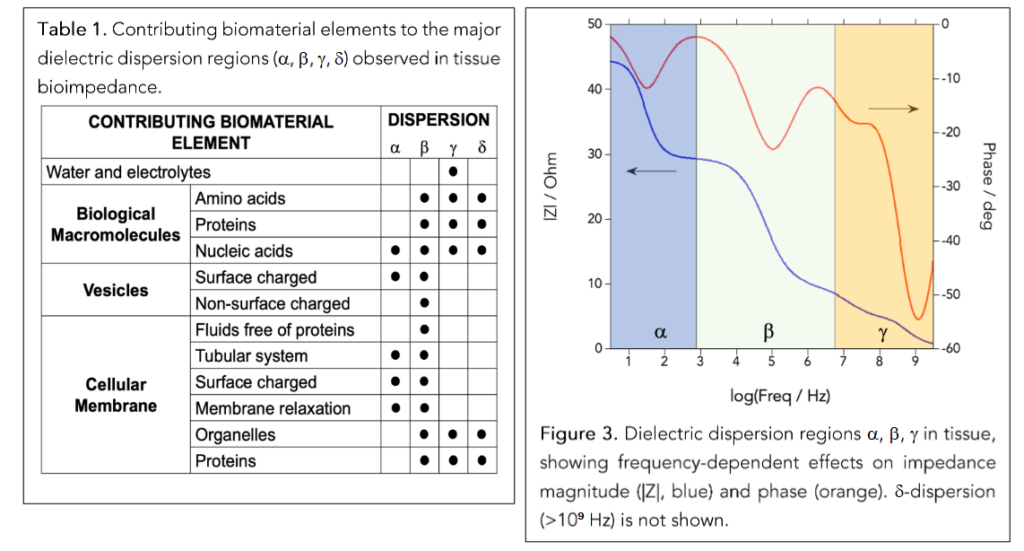
Table 1⁴³˒⁴⁴ represents a matrix of biomaterial elements that contribute to electrical dispersion in biological tissues, categorized by their influence on four dispersion regions: α, β, γ, and δ. These dispersion regions correspond to different frequency ranges in BIS.¹⁴ Each biomaterial element interacts with the applied electric field differently, depending on its structure and composition. Figure 3 shows the typical impedance spectrum over a logarithmic frequency range. The spectrum is divided into α, β, γ, and δ dispersion regions, each corresponding to a particular biophysical interaction. In the α region (low frequencies), the electric fields are primarily interacting with large-scale structures such as cell membranes and surface charges. In the β region (mid frequencies), impedance changes reflect increased current penetration through intact cells, often driven by capacitive charging of membranes and access to intracellular compartments. This is the region of interest for the discrimination between cancer and non-cancer cells. The γ region (higher frequencies) is where impedance is dominated by the dielectric relaxation of proteins, organelles, and smaller molecular structures. Distinct biological components contribute to the frequency-dependent impedance behavior, a principle that underlies the use of impedance spectroscopy for differentiating healthy and cancerous tissues based on their cellular and molecular composition.

The Cole-Cole Model and The Cole Relaxation Frequency

The measurement of electrical impedance in biological tissues is commonly modeled using the Cole-Cole equation, a mathematical representation that describes the dispersion of impedance as a function of frequency. First introduced by Kenneth Cole in the 1940s, this model characterizes the impedance behavior of biological systems using a set of parameters, including the Cole relaxation frequency (CRF), which represents the frequency at which the transition from capacitive to resistive behavior occurs.⁴⁵ The equation for impedance in the Cole-Cole model is given as:

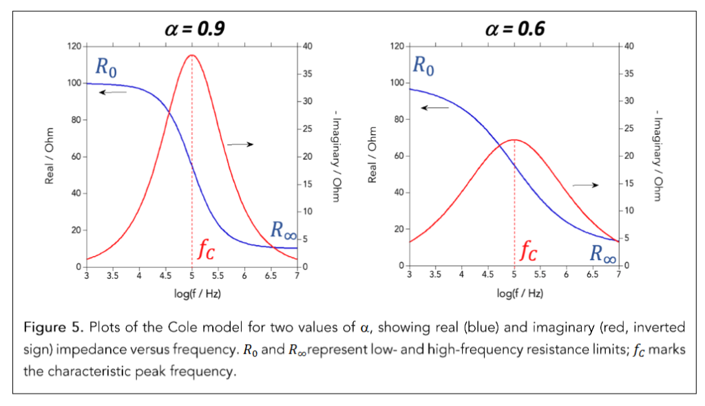
Z₍cole₎ = R∞ + (R₀ − R∞) / (1 + (j f / f_c)ᵅ)

where Z is the complex impedance, R₀ and R∞ are the low- and high-frequency resistance, respectively, f is the applied frequency, f_c is the Cole relaxation frequency (CRF), and α is a dispersion parameter that accounts for broadening effects in the impedance spectrum.

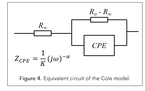
Figure 4. Equivalent circuit of the Cole model.

Figure 4 illustrates the electrical equivalent circuit of the Cole-Cole model, which is commonly used to represent the impedance characteristics of biological tissues. In this model, a resistor R∞ is placed in series with a parallel combination of a resistor R₀ and a Constant Phase Element (CPE). The CPE, in this context, models explicitly the behavior of the cellular membrane, which acts as an imperfect capacitor due to its complex structure and inhomogeneous properties.⁴⁶ Unlike an ideal capacitor (α = 1), the CPE exhibits a constant phase shift between voltage and current, capturing the distributed relaxation times typical of biological membranes. The characteristic parameter of the CPE is K, which represents the fractional capacitance and α (with values between 0 and 1) reflects the degree of deviation from ideal capacitive behavior. The Cole-Cole model of Equation 1 is the phenomenological representation of the equivalent circuit model of Figure 4, where the experimental parameters R₀, R∞, f_c, and α are directly extracted from the impedance spectra (Figure 5).

As we will demonstrate in this review, research has consistently shown that cancerous tissues exhibit higher CRF values than their benign or normal tissue. This distinction arises from changes in membrane polarization, altered ion transport dynamics, and increased intracellular conductivity. These physiological alterations shift the frequency-dependent impedance response, making CRF a powerful diagnostic indicator of malignancy. As such, CRF enables quantitative, non-invasive pathological assessment without the need for histological processing.

---

Correlating Breast Cancer with the Cole Relaxation Frequency

Early data were acquired from breast tissue excised during surgeries performed at two large metropolitan hospitals in the Midwestern United States. The goal of this initial research was to identify a specific and reproducible correlation between bioelectrical impedance measurements and the presence of breast cancer. At the time—approximately 25 years ago—the literature offered no established model linking impedance behavior to malignant pathology.

A pivotal finding from this early work, referred to here as the “Eureka Moment” (in tribute to Archimedes), played a critical role in uncovering the relationship between the cancerous state and impedance characteristics. Figure 6 displays a plot of the peak frequency of the reactive (imaginary) component of impedance as a function of frequency. On the left side of Figure 6, the horizontal axis shows a linear scale corresponding to the peak width, while the vertical axis uses a logarithmic scale to represent the peak frequency. Data points denote three distinct tissue categories, each confirmed through histological analysis: cancerous tissue, benign tissue, and adipose/fibro glandular breast tissue.

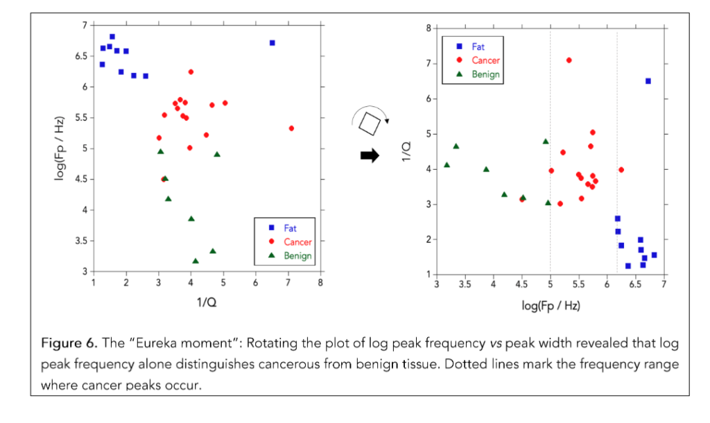
Initially, the width of the impedance peak appeared to offer little diagnostic value. Instead, it introduced additional variability, reducing the clarity of any observable correlation. Although later evaluations suggested that peak width may have conditional relevance, this early result highlighted a broader methodological concern: many previous approaches relied on interdependent parameters, increasing the risk of spurious associations and false diagnostic signals.

Nonetheless, while the original plot suggested only a modest grouping of tissue types, a clearer separation emerged after a geometric rotation of the data (as indicated by the arrow in Figure 6). In the transformed view, cancerous samples clustered predominantly within a frequency range of approximately 100 kHz to 2 MHz. This observation underscored the diagnostic potential of peak frequency as a robust and independent discriminator of malignancy.

Breast Cancer Diagnosis

METHODS

Impedance measurements were conducted on ex-vivo breast tissue specimens from 187 surgical patients using a commercial Solartron analyzer. Ag-AgCl or blackened platinum (BPt) electrodes were arranged in a four-terminal configuration. Frequency sweeps ranged from 1 Hz to 32 MHz, logarithmically spaced with 6–10 frequencies per decade. Cole relaxation frequencies were extracted from the spectra and correlated with each specimen’s pathology (cancerous vs noncancerous).

RESULTS
Analysis of the impedance measurements revealed that the Cole relaxation frequency (CRF) correlated strongly with the presence or absence of cancer in breast tissue specimens. When used as a single classifier in receiver operating characteristic (ROC) curve analysis, CRF achieved a sensitivity of 100% (95% CI: 99%–100%) and a specificity of 85% (95% CI: 79%–91%). These results indicate that CRF alone can be a highly effective discriminator between malignant and non-malignant breast tissues.

The application of CRF in breast cancer detection has been extensively investigated through both ex-vivo and in-vivo studies.¹⁶˒²² Early research involving impedance measurements on freshly excised breast tissue samples revealed that malignant tissues exhibited CRF values up to 1000 times higher than benign tissues, suggesting a clear electrical signature associated with cancerous transformation. In a study by Gregory,¹⁶ the use of CRF as a diagnostic parameter was found to achieve high sensitivity and specificity, supporting its potential as a reliable classifier for distinguishing malignant from non-malignant breast lesions.

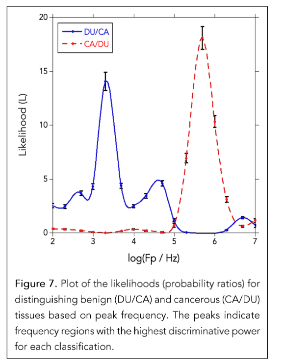
Figure 7 presents the likelihood ratio analysis of CRF measured in excised breast tissue, showing how well specific frequency ranges distinguish between cancerous (CA) and ductal (DU) tissue.²⁰ The likelihood (L) was calculated by taking the ratio of normalized frequency distributions: P(f | CA)/P(f | DU) for the red dashed curve (CA/DU), and P(f |DU) / P (f | CA) for the blue solid curve (DU/CA). This analysis revealed two distinct frequency regions: one centered around 10³ to 10⁴ Hz where DU tissue is far more likely, and another near 10⁵ to 2 × 10⁶ Hz where CA tissue dominates. Importantly, the peaks of CA/DU and DU/CA are separated by more than two orders of magnitude in frequency, highlighting a clear spectral distinction between cancerous and normal tissue. These results strongly support the notion that the Cole relaxation frequency alone—without relying on other parameters—can effectively differentiate cancerous from non-cancerous breast tissue with high sensitivity and specificity.

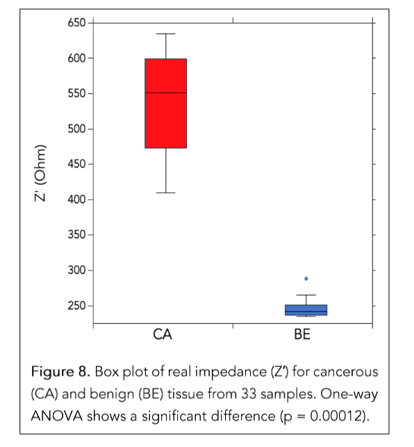
Figure 8 shows a box plot of a reduced dataset of 33 impedance samples measured over the frequency range from 1 kHz to 3.2 MHz. In the study by Shell and Gregory,⁴⁷ this dataset was used for a one-way ANOVA after removing the lowest and highest frequency data to avoid distortions from electrode polarization and noise. The ANOVA revealed a p-value of 0.00012, which is far below typical significance thresholds, confirming that the mean impedance values of malignant and benign tissues differ significantly across the selected frequency range. This analysis complemented other non-parametric tests like the Kolmogorov-Smirnov and Kruskal-Wallis, all converging on the same conclusion: the tissue types have statistically distinct impedance characteristics suitable for machine learning classification.

Building upon these results, the authors implemented a multi-tiered neural network (NN) approach designed to enhance diagnostic accuracy.⁴⁷ The motivation for using neural networks was to leverage their powerful pattern recognition capabilities, particularly effective at identifying complex, nonlinear relationships in bioimpedance data. The strategy involved six distinct backpropagation neural networks, each using different optimization techniques, including Gradient Descent, Levenberg-Marquardt, and Resilient Backpropagation. These networks were rigorously trained, validated, and tested using impedance data collected from excised breast tissue samples.

The neural networks demonstrated remarkable diagnostic performance, achieving perfect sensitivity (100%) and specificity (100%) on a dataset consisting of 180 malignant and 180 benign samples. These results underscore the clinical potential of neural networks in interpreting intricate bioimpedance data, providing an efficient, objective, and non-invasive diagnostic aid. Visualizations of network output (e.g., Figures 13 and 15 of reference 23) confirmed the strong separation between tissue types, and regression plots demonstrated a high correlation (R ≈ 0.99) between predicted and actual labels during training and validation.

From a clinical perspective, the integration of advanced neural network techniques with impedance spectroscopy could significantly improve cancer diagnostics by enabling rapid and accurate assessments. This approach could be particularly impactful in settings with limited diagnostic resources, supporting more timely and precise clinical decision-making.

The study demonstrates the analytical robustness and clinical promise of combining rigorous statistical validation with advanced neural network models,

positioning bioimpedance spectroscopy as a valuable diagnostic tool for breast cancer detection and management.

Breast Cancer Prognosis

METHODS

This retrospective study,²¹ approved by the institutional review board, followed up on a prior clinical study (2003–2012)¹⁶ in which 187 patients underwent intraoperative impedance measurements during excision of benign and malignant breast lesions. For this analysis, 108 patients with confirmed malignancies and long-term follow-up records in the Aurora Health Care cancer registry were included. Among them, 84 had no recurrence, and 24 experienced recurrence, including 7 with metastasis.

CRF values were extracted intraoperatively and normalized by 100 kHz to produce a dimensionless parameter (nCRF, range: 1–20), enabling frequency-based recurrence risk stratification. Exceedance averaging estimated cancer-free survival as a function of nCRF, with values below or above thresholds weighted as 0 or 1, respectively. The same method was applied to the Nottingham Prognostic Index (NPI)⁴⁸ for comparison.

Outcome-specific nCRF distributions—no recurrence (NR), recurrence without metastasis (RNM), and recurrence with metastasis (RM)—were used to define three diagnostic regions: L-NR (nCRF < 3), L-RNM (3 ≤ nCRF ≤ 6), and L-RM (nCRF > 6). Likelihood ratios (e.g., L(f) = P(f | RM) / P(f | NR)) guided segmentation, and t-tests assessed separability between regions.

Multivariate Cox proportional hazards models⁴⁹ compared nCRF to NPI and tumor grade, adjusting for age and biomarker status (ER, PR, HER2/neu). Hazard ratios with 95% confidence intervals were reported using SAS 9.4.

RESULTS

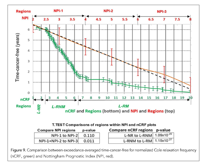
Figure 9 presents a comparison between nCRF and the NPI using an exceedance averaging method, which estimates the expected duration of cancer-free survival as a function of each prognostic variable. The green curve representing nCRF displays three well-defined regions with distinct breakpoints. Values of nCRF below 3 correspond to patients who remained recurrence-free, values between 3 and 6 indicate recurrence without metastasis, and values above 6 are associated with metastatic recurrence. The red curve, corresponding to NPI, lacks sharp boundaries and shows only a gradual change across regions. Statistical comparisons show partial separation among NPI regions, with NPI-1 and NPI-2 not significantly different (p = 0.110), while NPI-2 and NPI-3 are marginally distinct (p = 0.011). In contrast, nCRF separates all three outcome groups with statistical significance (p < 10⁻²⁰). These findings highlight the utility of nCRF as a more precise and discriminative prognostic parameter than traditional indices, offering a quantitative, non-invasive method for predicting recurrence risk and metastatic potential in breast cancer.

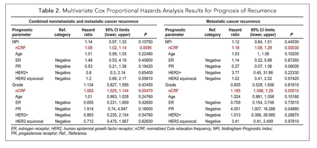
Table 2. Multivariate Cox Proportional Hazards Analysis Results for Prognosis of Recurrence

Table 2 presents the results of a multivariate Cox proportional hazards analysis evaluating various prognostic parameters for predicting time-cancer-free survival in breast cancer patients. The analysis includes two outcome categories: combined recurrence (recurrence with or without metastasis) and metastatic recurrence only. Each model adjusts for multiple clinical factors, including age, estrogen receptor (ER) status, progesterone receptor (PR) status, HER2/neu status, and either the NPI or tumor grade, depending on the comparison.

The nCRF stands out as the only parameter consistently and significantly associated with worse outcomes in both categories. For combined recurrence, nCRF showed a hazard ratio (HR) of 1.08 with a p-value of 0.0095 (when compared to NPI) and p = 0.0047 (when compared to grade). For metastatic recurrence, nCRF had a stronger HR of 1.185, with p-values of 0.0003 (vs NPI) and 0.0001 (vs grade), indicating that higher nCRF values were significantly associated with increased risk of recurrence and metastasis.

In contrast, traditional prognostic markers like NPI, grade, ER, PR, HER2/neu, and age was not statistically significant in most comparisons. The only marginally significant result among these was a higher risk of metastatic recurrence associated with PR-negative status (HR = 4.05, p = 0.0488), though this was not observed for combined recurrence. Overall, the table supports nCRF as a superior and independent prognostic indicator compared to commonly used clinical parameters.

In-vivo Breast Cancer Imaging and Mapping

METHODS

To localize malignancies based on spatial variations in Cole Relaxation Frequency (CRF), a mammography-compatible device with a 256-electrode array collected impedance data during breast compression from 50 patients.²² Impedance spectra (10 kHz–1 MHz) were fit to the Cole model at each electrode to extract CRF values. Malignant tissue consistently exhibited CRF values above 100 kHz, enabling both binary classification and spatial mapping without the need for signal inversion or tomographic reconstruction. The method successfully identified and localized cancerous regions in agreement with pathology, demonstrating feasibility for radiation-free breast cancer screening.

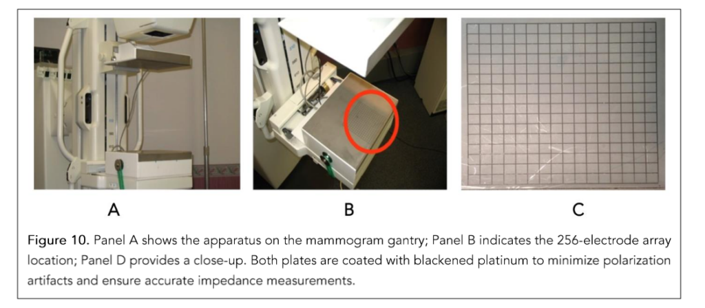
Figure 10 shows the hardware setup mounted on a standard mammography gantry. The Drive Plate (top) applied 1 V RMS across all frequencies, while the Electrode Plate (bottom) was grounded and featured a 16 × 16 array (256 total electrodes) to measure local current response, enabling spatially resolved impedance mapping of the compressed breast surface.

RESULTS

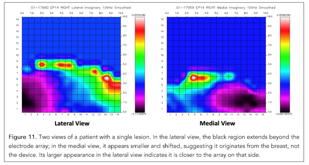
Figure 11 illustrates how the CRF-based imaging technique identifies and maps cancerous regions. The two scans were obtained by rotating the gantry 180° from a lateral to a medial view. Note that the black anomalous region—later confirmed by biopsy as a cancerous tumor—shifts from left to right between views. This comparison confirms that the observed features originate from the breast and are not artifacts of the device. Moreover, the anomaly also appears larger in the lateral view, suggesting that the tumor is closer to those electrodes and not deeply embedded in the breast tissue.

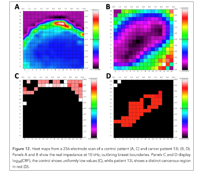
Figure 12. Heat maps from a 256-electrode scan of a control patient (A, C) and cancer patient 13L (B, D). Panels A and B show the real impedance at 10 kHz, outlining breast boundaries. Panels C and D display log₁₀(CRF); the control shows uniformly low values (C), while patient 13L shows a distinct cancerous region in red (D).

Figure 12 compares results from a control patient (no cancer) and patient 13L (diagnosed with cancer). Subfigures (A) and (B) display the real part of the impedance at 10 kHz across the 256 electrodes, which helps visualize the physical boundary of the breast. Subfigures (C) and (D) show the CRF values log₁₀(f_c) at each electrode. In the control patient, CRF values remain consistently low (non-cancerous), whereas, for patient 13L, a specific region appears with CRF > 100 kHz, indicating cancerous tissue.

This demonstrates how spatial variations in CRF can effectively localize malignancies without requiring signal inversion or tomographic reconstruction, offering a simple and direct visualization of cancer within the breast.

These results validate the use of CRF as a spatially resolved diagnostic signal capable of identifying and localizing malignant regions in the breast. The clear contrast in CRF patterns between healthy and cancerous tissue

cancerous tissue, as observed across multiple views and in comparison to pathology, supports the technique’s reliability and reproducibility. Unlike traditional imaging modalities, this approach does not rely on ionizing radiation or complex tomographic reconstruction, offering a rapid, patient-friendly alternative for real-time tissue characterization.

Electrical Property Enhanced Tomography

Extending impedance-based cancer detection to 3D imaging is limited by the instability of traditional Electrical Impedance Tomography (EIT),⁵⁰ where small signal errors can lead to large image distortions due to the ill-posed inverse problem.

Electrical Property Enhanced Tomography (EPET) addresses this by integrating anatomical imaging (e.g., CT or MRI) to define tissue boundaries,⁵¹ then overlaying impedance data onto these segmented maps. This structured formulation, using orthogonal basis functions like sine or Bessel modes, creates a well-conditioned system. With regular electrode geometry and smooth tissue segmentation, EPET reduces error propagation by up to 100-fold, enabling precise and clinically robust impedance imaging.

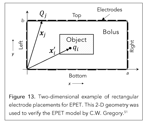
Figure 13. Two-dimensional example of rectangular electrode placements for EPET. This 2-D geometry was used to verify the EPET model by C.W. Gregory.⁵¹

Figure 13 illustrates the core geometry used in EPET. A rectangular electrode array surrounds the object under test, separated by an electrically conductive bolus that enhances coupling between the electrodes and tissue. This bolus ensures consistent contact, minimizes contact impedance artifacts, and maintains a uniform current distribution. The field point and source point notation (xᵢ′ and xⱼ) used in the mathematical formulation supports the derivation of Green’s function-based integral equations. This arrangement allows EPET to model the potential field inside the object using Fourier-based methods, which provide high accuracy and reduce error sensitivity in the forward and inverse solutions.⁵²

According to Maxwell’s equations, external electrode charges are intrinsically linked to internal charge distributions. Internal charge accumulations arise at boundaries where conductivity or permittivity changes abruptly—except when the boundary is perpendicular to the electric field, where no buildup occurs. As a result, induced charge patterns form around internal anomalies, such as anatomical structures or tumors, reflecting local dielectric and conductive contrasts.

A key advantage of the EPET approach lies in its use of a spatial Fourier transform to convert the raw boundary measurements into an orthogonal mode representation. When the electrodes are evenly spaced along a rectangular boundary, the surface charge distribution Q(x) can be expressed as a discrete sine series, where its coefficients are computed via a discrete sine transform:

Aₗ = (2/a) Σⱼ₌₁ᴺ Q(xⱼ) · sin(ℓπxⱼ / a)

Aₗ represents the amplitude of the ℓ-th spatial frequency mode, a is the length of the x-axis side of the rectangular box, and xⱼ are the electrode positions. This transformation yields a vector A = (A₁, A₂, …, Aᴹ)ᵀ that characterizes the observed data.

The internal charge distribution δq = (δq₁, δq₂, …, δqᴹ)ᵀ is then related to these Fourier coefficients through the linear expression:

A = B · δq

Here, the matrix B is constructed from sine and hyperbolic sine terms derived from the Green’s

function solution to the forward problem (Maxwell’s equations) and each element of B has the form²⁵:

Bₗ,ᵢ = sin(ℓπxᵢ′ / a) · [ sinh(ℓπ(b − yᵢ′) / a) / sinh(ℓπb / a) ]

where (xᵢ′, yᵢ′) are the coordinates of the i-th internal voxel, and b is the length of the y side of the box. This formulation encapsulates the spatial influence of each internal charge element on each Fourier mode of the boundary measurement.

If the matrix B is full-rank and well-conditioned—which is typically achieved under ideal electrode placement and anatomical segmentation—then the internal charge distribution can be recovered by inverting the system:

δq = B⁻¹ · A

This transformation from spatial data to Fourier mode space and the associated inversion of B is what enables EPET to reconstruct internal charge patterns with high spatial fidelity and robustness to noise. The use of orthogonal basis functions ensures that each mode contributes independently and the near-identity condition B⁻¹ · B ≈ I confirms that the inversion does not amplify errors (Figure 14-A).

To further improve the stability and accuracy of the inverse solution in EPET, particularly under realistic conditions involving measurement noise or imperfect electrode alignment, the Singular Value Decomposition (SVD)⁵³ method can be employed. SVD factorizes the system matrix, allowing for the computation of a pseudoinverse B⁻¹, which can be used to recover the internal charge distribution from Fourier-transformed measurements via:

δq = B⁻¹ · A

When applied to the EPET system, the use of SVD results in a matrix product B⁻¹ · B that more closely approximates the identity matrix, indicating a significantly improved inversion accuracy and numerical stability. The reduction of residual off-diagonal elements further confirms the enhanced orthogonality and robustness of the system (Figure 14-B).

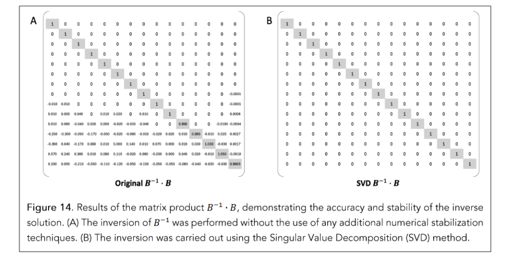
Figure 14. Results of the matrix product B⁻¹ · B, demonstrating the accuracy and stability of the inverse solution. (A) The inversion of B⁻¹ was performed without the use of any additional numerical stabilization techniques. (B) The inversion was carried out using the Singular Value Decomposition (SVD) method.

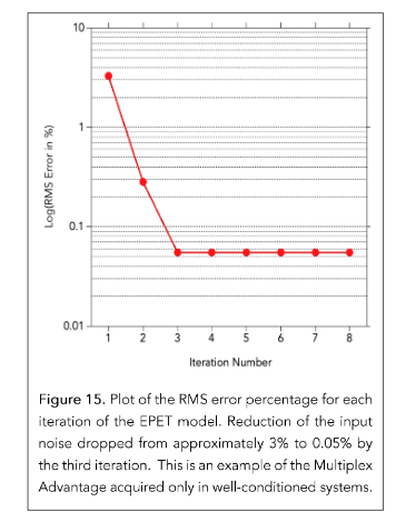
Figure 15. Plot of the RMS error percentage for each iteration of the EPET model. Reduction of the input noise dropped from approximately 3% to 0.05% by the third iteration. This is an example of the Multiplex Advantage acquired only in well-conditioned systems.

Figures 15 demonstrate the practical impact of this modeling framework. It plots the logarithm of the root-mean-square (RMS) error between the true and estimated electrical property values across successive iterations of the inverse solution using the Iterative Correction Method. After only three iterations, the method converges to within 0.05% RMS error, even when simulated measurement noise of ~1% is added to the input data. When no noise is introduced, the model converges to the true values with double-precision accuracy.

This mathematical structure is central to the stability and precision of EPET reconstructions, distinguishing it fundamentally from conventional EIT approaches. These findings confirm that the inverse solution remains stable and exhibits robust convergence, even when the initial estimates of tissue properties deviate significantly from their true values. In practice, this implies that EPET can generate highly accurate maps of conductivity and permittivity even under non-ideal clinical conditions, such as patient movement or measurement noise.

The integration of anatomical priors, structured electrode design, and well-conditioned mathematical inversion makes EPET a powerful technique for functional imaging, capable of reliably detecting cancer-associated alterations in tissue electrical properties.

---

Application to Intraoperative Skin Cancer Detection

Bioelectrical impedance spectroscopy (BIS) offers rapid, non-destructive skin cancer detection and is particularly useful in Mohs micrographic surgery (MMS). Although frozen section histology is the clinical standard for margin assessment, it is slow (20–40 minutes) and destructive, limiting its use for real-time surgical decisions.⁵⁴

High-frequency BIS (HF-BIS) can detect malignant vs non-malignant tissue within 3–5 minutes, providing actionable information during surgery. Beyond skin cancer, this method has strong potential for breast-conserving procedures, where real-time margin detection is essential to spare healthy tissue.

Effective BIS-based margin assessment requires resolving cancer within thin surgical margins. This imposes strict constraints on electrode design and current field geometry. Unlike deep imaging, superficial margin detection demands shallow, well-confined current penetration to localize pathology at the tissue surface.⁵⁵

 

METHODS

A custom bipolar planar electrode array with closely spaced Ag/AgCl electrodes was designed to achieve shallow current penetration for margin assessment in dermal samples. A conductive gel ensured effective coupling between electrodes and tissue. Impedance data were acquired from 1 kHz to 20 MHz using a customized analyzer.

To quantify current confinement, depth profiles were measured using stepper motors and tissue phantoms positioned above the electrodes embedded in the gel.

A multi-feature machine learning (ML) classifier was trained on impedance data labeled with histology-confirmed annotations. Prediction heatmaps were generated from spatially registered measurements.

The model was validated using 5-fold cross-validation and evaluated by sensitivity, specificity, and area under the ROC curve (AUC).

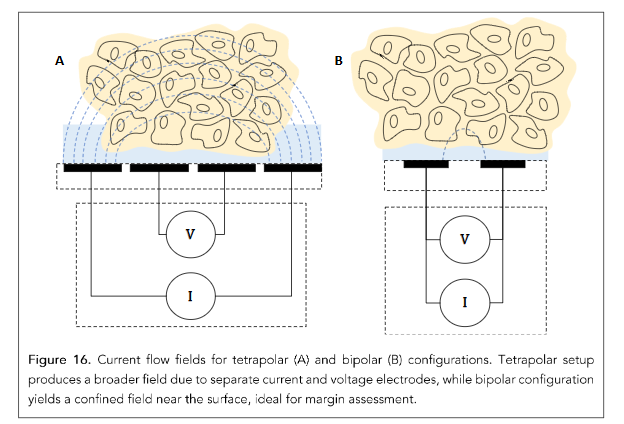
Figure 16. Current flow fields for tetrapolar (A) and bipolar (B) configurations. Tetrapolar setup produces a broader field due to separate current and voltage electrodes, while bipolar configuration yields a confined field near the surface, ideal for margin assessment.

---

RESULTS

Figure 16 illustrates the difference between tetrapolar and bipolar electrode configurations. While tetrapolar setups reduce polarization and contact resistance, they generate diffuse fields with deep penetration—unsuitable for thin-margin detection. In contrast, the bipolar configuration, enabled by low-polarization Ag/AgCl electrodes, produces tightly confined fields ideal for detecting superficial cancer near the tissue edge. Figure 17 quantifies current density across three electrode spacings. At 0.5 mm spacing, 90% of the current is confined within ~600 µm, confirming that shallow, localized penetration is achievable with optimized array design. Figure 18 shows the custom-fabricated electrode array designed for margin assessment. Bipolar pairs arranged in a grid enable spatially resolved impedance measurements across the specimen surface, achieving ~0.5 mm resolution suitable for clinically relevant heatmaps.

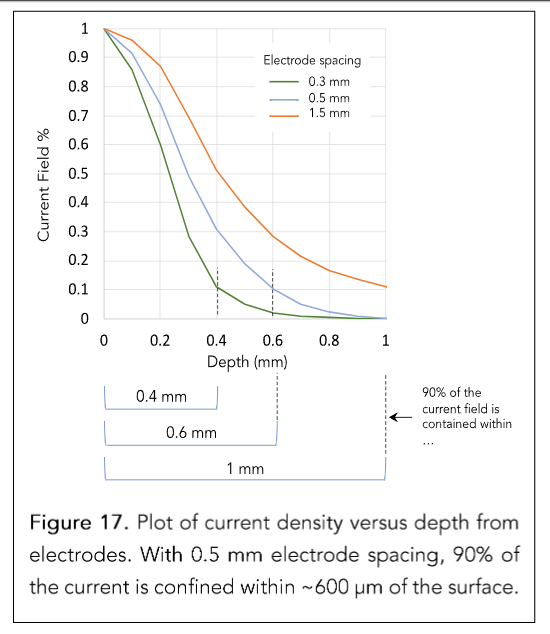
Figure 17. Plot of current density versus depth from electrodes. With 0.5 mm electrode spacing, 90% of the current is confined within ~600 µm of the surface.

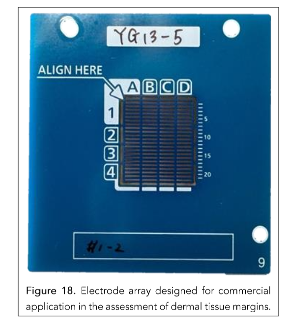
Figure 18. Electrode array designed for commercial application in the assessment of dermal tissue margins.

By combining optimized electrode geometry, shallow field confinement, and robust data acquisition, the system provides real-time, high-resolution guidance that can guide tissue-sparing surgeries in both skin and breast cancer.

One of the key challenges in applying BIS to skin cancer detection is the heterogeneous nature of skin tissue.⁵⁶ Composed of multiple layers—epidermis, dermis, subcutaneous fat—and structures like glands and follicles, skin exhibits wide variability in electrical properties.⁵⁶˒⁵⁷ These differences, compounded by hydration, vascularization, inflammation, and fibrosis, make it difficult to set fixed thresholds for distinguishing benign from malignant tissue. Additionally, while clinical standards define a positive margin as carcinoma within 300 µm of the tissue edge, the device detects impedance changes up to 600 µm deep. Without selective interpretation, this added depth could produce clinically irrelevant signals.

To overcome these limitations, a machine learning (ML) model was trained on histology-labeled data to mimic the surgeon’s interpretive standard. Although the device senses deeper electrical changes, the ML model is trained to focus on impedance patterns associated with carcinoma within the top 300 µm—effectively filtering out non-actionable signals from deeper regions. This ensures that its predictions reflect what a Mohs surgeon would consider a positive margin.

Importantly, the ML model also improves signal selectivity, distinguishing cancer-specific impedance features from those of normal or inflamed skin structures and enhancing diagnostic accuracy.

Figure 19 demonstrates this capability: a spatial heatmap generated by the trained model closely matches the histological margin defined by Toluidine Blue–Metachromatic Blue staining.⁵⁸ The high-probability cancer region aligns with the confirmed carcinoma, underscoring the model’s precision and clinical relevance.

Validation of the ML model’s performance is presented in Figure 20, which includes a box plot of prediction probabilities and the corresponding receiver operating characteristic (ROC) curve for cancer detection at the location level. The model underwent 5-fold cross-validation, achieving 91% sensitivity and 96% specificity at the individual electrode level. The ROC curve yields an area under the curve (AUC) of 0.93 ± 0.02, indicating high diagnostic accuracy and robustness across five-fold cross-validation. The tight confidence band highlights model consistency across folds, even under natural variations in tissue properties.

These results confirm that AI-enhanced impedance analysis significantly improves diagnostic performance. By learning from complex tissue variability, the ML model enables accurate, real-time localization of carcinoma without compromising tissue integrity. This approach offers a powerful tool for intraoperative margin assessment in both skin and breast cancer surgeries, where preserving healthy tissue while ensuring complete tumor removal is paramount. The successful application of this technology in skin cancer provides strong evidence that a similar real-time, ML-guided EIS strategy could dramatically improve margin evaluation and reduce re-excision rates in breast-conserving procedures.

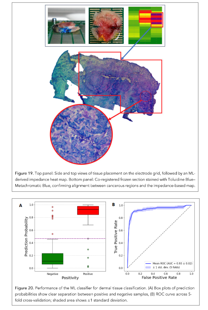
Figure 19. Top panel: Side and top views of tissue placement on the electrode grid, followed by an ML-derived impedance heat map. Bottom panel: Co-registered frozen section stained with Toluidine Blue–Metachromatic Blue, confirming alignment between cancerous regions and the impedance-based map.

Figure 20. Performance of the ML classifier for dermal tissue classification. (A) Box plots of prediction probabilities show clear separation between positive and negative samples, (B) ROC curve across 5-fold cross-validation; shaded area shows ±1 standard deviation.

Discussion

The body of work presented in this review demonstrates the substantial diagnostic and prognostic value of bioelectrical impedance spectroscopy (BIS) and the Cole Relaxation Frequency (CRF) in cancer detection and management. From the initial discovery of CRF as a marker that differentiates malignant from benign breast tissue through rigorous statistical validation and advanced modeling to the development of real-time imaging and intraoperative assessment tools, this technology has evolved into a clinically relevant diagnostic platform.

In breast cancer, CRF has proven to be a robust and non-invasive diagnostic indicator. It not only distinguishes cancerous from non-cancerous tissue with high sensitivity and specificity but also offers meaningful prognostic insights. Elevated CRF values correlate with an increased risk of recurrence and metastasis, outperforming traditional markers such as the Nottingham Prognostic Index. The use of normalized CRF (nCRF) enables clearer stratification of patient outcomes, offering clinicians a quantitative parameter to guide treatment planning and risk assessment.

The introduction of Electrical Property Enhanced Tomography (EPET) has addressed a key limitation of traditional Electrical Impedance Tomography (EIT): instability caused by noise in solving the inverse problem. By combining anatomical imaging with impedance measurements and modeling the solution using orthogonal basis functions, EPET achieves nearly two orders of magnitude reduction in noise propagation. This significantly enhances the accuracy and spatial resolution of impedance-based imaging and makes three-dimensional tissue mapping feasible for clinical use.

In the surgical setting, particularly in skin and breast cancer procedures, real-time intraoperative assessment of margins is essential to minimizing re-excision while preserving healthy tissue. The use of miniaturized, high-resolution electrode arrays, as demonstrated in the assessment of dermal tissue, enables precise current confinement within superficial margins of interest. The adoption of a bipolar electrode configuration, made possible by advanced Ag/AgCl fabrication with low polarization, allows for shallow and well-localized electric fields ideal for margin assessment. This technological refinement ensures that carcinoma can be detected within a few hundred microns from the tissue edge—critical for tissue-sparing operations like lumpectomies and Mohs surgery.

Finally, the integration of artificial intelligence (AI) and machine learning (ML) into impedance analysis has proven transformative. Trained ML models offer high sensitivity and specificity while maintaining robustness across variable tissue conditions. By leveraging AI, these systems can overcome the natural electrical variability in heterogeneous tissues like skin and breast, enabling fast, reliable, and objective margin assessments during surgery.

Conclusion

Taken together, these innovations position CRF-based impedance analysis as a powerful tool across the cancer care continuum—from non-invasive detection and in-vivo mapping to prognostic stratification and intraoperative guidance. The approach offers real-time feedback, preserves tissue integrity, and holds promise to reduce both the time and cost of cancer diagnosis and treatment. As integration with clinical workflows advances, this technology could play a central role in improving outcomes through more personalized, efficient, and minimally invasive care.

Although each application discussed in this review was conducted under institutional ethical oversight, broader clinical adoption will require prospective, multi-center trials to validate performance, generalizability, and impact on patient outcomes. It is the authors’ hope that such studies will be undertaken in the near future, enabling this promising technology to transition from research to routine clinical practice—ultimately supporting better clinical practice.

informed surgical decisions and more precise cancer management.

Funding:

This material is based upon work supported in part by the National Science Foundation under Award Numbers 0944454 and 1058413. Any opinions, findings, conclusions, or recommendations expressed in this publication are those of the authors and do not necessarily reflect the views of the National Science Foundation. Additional support was provided by the University of Wisconsin–Milwaukee; Aurora Health Care Inc.; NovaScan, Inc.; the Wisconsin Institute for Biomedical and Healthcare Technologies; and CAMCARE, the research and education foundation of the Charleston Area Medical Center, Charleston, WV. A portion of this work was also supported by WiSys, a subsidiary of the Wisconsin Alumni Research Foundation, and the University of Wisconsin System.

Acknowledgments:

We are grateful to our colleagues at the University of Wisconsin–Milwaukee (Shabistan Sheerin), Marquette University (Cory Steinmetz), Aurora Health Care (Carol Davis and Carol Halliday), and NovaScan (Paul Voith, Alan Nichols, and Shahila Mehboob Christie) for their assistance. Urs Reuteler contributed the illustration for Figure 10. Sean Gregory provided valuable help with the MATLAB calculations for Figure 11.

In Memoriam:

We regretfully acknowledge the contributions of our long-time collaborator and co-author, John R. Shell. John retired to the Dominican Republic a few years ago and passed away shortly thereafter. Rest in peace, John.

Table 2 and Figure 9 are used under Free License from the copyright owner (the Journal of Patient Centered Research and Reviews) with the Authors Gregory WD, Christie SC, Shell J, Nahhas GJ, Singh M, Mikkelson W. Title: Cole relaxation frequency as a prognostic parameter for breast cancer. Source: Patient Cent Res Rev. 2020;7:343–8. doi: 10.17294/2330-0698.1794

Figures 10 and 12 are images by – Authors: Gregory WD, Christie SM, Gregory CW, Marx JJ, Shell J, Wendy Mikkelson, Title: The Cole Relaxation Frequency as a Parameter to Identify and Spatially Map Cancer in Breast Tissue: Preliminary In-Vivo Patient Study. Source: Trans Biomed Vol.12 No.9:192, available at https://www.transbiomedicine.com/, Licensed Under License of Creative Commons Attribution 3.0 License

Conflicts of Interest:

Certain intellectual property related to the results reported here has been assigned by the University of Wisconsin–Milwaukee to WiSys, a subsidiary of the Wisconsin Alumni Research Foundation (WARF), the patent licensing arm of the University of Wisconsin System. WiSys has, in turn, granted an exclusive license for this intellectual property to NovaScan, Inc. W.D. Gregory, C.W. Gregory, and Aurora Health Care have financial interests in NovaScan LLC. However, Aurora Health Care personnel J.J. Marx and W. M. Mikkelson have no financial interest derived from this relationship.

 

References

1. Sung H, Ferlay J, Siegel RL, et al. Global Cancer Statistics 2020: GLOBOCAN Estimates of Incidence and Mortality Worldwide for 36 Cancers in 185 Countries. CA Cancer J Clin. 2021;71(3): 209-249.

2. Crosby D, Bhatia S, Brindle KM, et al. Early detection of cancer. Science. 2022;375(6586):eaay 9040.

3. Harbeck N, Penault-Llorca F, Cortes J, et al. Breast cancer. Nat Rev Dis Primers. 2019;5(1):66. Published 2019 Sep 23.

4. Bonotto M, Gerratana L, Poletto E, et al. Measures of outcome in metastatic breast cancer: insights from a real-world scenario. Oncologist. 2014;19(6):608-615.

5. Hu M, Shao B, Ran R, Li H. Prognostic factors for patients with metastatic breast cancer: a literature review. Transl Cancer Res. 2021;10(4): 1644-1655.

6. Lord SJ, Bahlmann K, O’Connell DL, et al. De novo and recurrent metastatic breast cancer – A systematic review of population-level changes in survival since 1995. EClinicalMedicine. 2022;44: 101282. Published 2022 Jan 29.

7. DeSantis CE, Ma J, Gaudet MM, et al. Breast cancer statistics, 2019. CA Cancer J Clin. 2019;69(6):438-451.

8. Liu H, Zhan H, Sun D, Zhang Y. Comparison of BSGI, MRI, mammography, and ultrasound for the diagnosis of breast lesions and their correlations with specific molecular subtypes in Chinese women. BMC Med Imaging. 2020;20(1):98. Published 2020 Aug 15.

9. Tao Z, Qi H, Ma Y. Diagnostic efficacy of ultrasound elastography and dynamic contrast-enhanced MR in benign and malignant breast masses. Am J Transl Res. 2023;15(4):2870-2877. Published 2023 Apr 15.

10. Mayo, R. C., & Romero, A. (2020). Redefining the Use of Breast Imaging: Mammography, Ultrasound, and MRI in Dense Breasts and Breast Cancer Screening. American Journal of Roentgenology, 214(2), 295-306.

11. Dianatinasab M, Fararouei M, Mohammadianpanah M, Zare-Bandamiri M. Impact of social and clinical factors on diagnostic delay of breast cancer: A Cross-sectional Study. Medicine (Baltimore). 2016;95(38):e4704.

12. Aresta G, Araújo T, Kwok S, et al. BACH: Grand challenge on breast cancer histology images. Med Image Anal. 2019;56:122-139.

13. Yu F, Xiao Z, Liu L, et al. BiaCanDet: Bioelectrical impedance analysis for breast cancer detection with space–time attention neural network. Expert Systems with Applications. 2025;269:126 223.

14. Abasi S, Aggas JR, Garayar-Leyva GG, Walther BK, Guiseppi-Elie A. Bioelectrical Impedance Spectroscopy for Monitoring Mammalian Cells and Tissues under Different Frequency Domains: A Review. ACS Measurement Science Au. Published online August 19, 2022.

15. Branco MG, Mateus C, Capelas ML, et al. Bioelectrical Impedance Analysis (BIA) for the Assessment of Body Composition in Oncology: A Scoping Review. Nutrients. 2023;15(22):4792. Published 2023 Nov 15.

16. Gregory WD, Marx JJ, Gregory CW, Mikkelson WM, Tjoe JA, Shell J. The Cole relaxation frequency as a parameter to identify cancer in breast tissue. Med Phys. 2012;39(7):4167-4174.

17. Bogdanowicz L, Onur Fidaner, Ceres D, Grycuk A, Guidetti M, Demos D. The Cole Relaxation Frequency as a Parameter to Identify Cancer in Lung Tissue: Preliminary Animal and Ex-Vivo Patient Studies. JMIR Biomedical Engineering. 2022;7(1): e35346-e35346.

18. Svoboda RM, Gharia MJ, Shell J, Gregory WD. Bioimpedance measurement as an assessment of margin positivity in Mohs surgical specimens of nonmelanoma skin cancer: Management implications. J Am Acad Dermatol. 2018;79(3):591-593.

19. Federica Dibennardo, Onur Fidaner, Bogdanowicz L, et al. Bioimpedance based biomarker for the detection of precancerous and cancerous lesions of the pancreas: feasibility animal study. Translational medicine communications. 2024;9(1).

20. Bogdanowicz L, Guidetti M, Onur Fidaner, et al. S31 Cole Relaxation Frequency: A Parameter for Pancreatic Cancer Detection. The American Journal of Gastroenterology. 2022;117(10S):e24-e25.

21. Gregory WD, Christie SM, Shell J, Nahhas GJ, Singh M, Mikkelson W. Cole Relaxation Frequency as a Prognostic Parameter for Breast Cancer. J Patient Cent Res Rev. 2020;7(4):343-348. Published 2020 Oct 23.

22. Gregory WD, Christie SM, Gregory CW, Marx JJ, Shell J, et al. (2021) The Cole Relaxation Frequency as a Parameter to Identify and Spatially Map Cancer in Breast Tissue: Preliminary In-Vivo Patient Study. Transl Biomed Vol.12 No.9:192

23. Stupin DD, Kuzina, Ekaterina A, Abelit AA, et al. Bio-Impedance Spectroscopy: Basics and Applications. arXiv.org. Published 2020.

24. Campa F, Coratella G, Cerullo G, et al. High-standard predictive equations for estimating body composition using bioelectrical impedance analysis: a systematic review. Journal of Translational Medicine. 2024;22(1).

25. Poßner L, Seebeck L, Laukner M, et al. A four-point measurement probe for brain tissue conductivity and permittivity characterization. Published online April 30, 2021.

26. Bera TK. Bioelectrical Impedance and The Frequency Dependent Current Conduction Through Biological Tissues: A Short Review. IOP Conference Series: Materials Science and Engineering. 2018; 331:012005.

27. Yu Y, Kalra AM, Anand G, Lowe A. A Pilot Study Examining the Dielectric Response of Human Forearm Tissues. Biosensors. 2023;13(11):961-961.

28. Moqadam SM, Grewal PK, Haeri Z, Ingledew PA, Kohli K, Golnaraghi F. Cancer Detection Based on Electrical Impedance Spectroscopy: A Clinical Study. J Electr Bioimpedance. 2018;9(1):17-23. Published 2018 Aug 16.

29. Rejniak KA, Estrella V, Chen T, Cohen AS, Lloyd MC, Morse DL. The Role of Tumor Tissue Architecture in Treatment Penetration and Efficacy: An Integrative Study. Frontiers in Oncology. 2013;3.

30. Zanotelli MR, Zhang J, Reinhart-King CA. Mechanoresponsive metabolism in cancer cell migration and metastasis. Cell Metab. 2021;33(7): 1307-1321.

31. Teixeira VS, Labitzky V, Schumacher U, Krautschneider W. Use of Electrical Impedance Spectroscopy to Distinguish Cancer from Normal Tissues with a Four Electrode Terminal Setup. Current Directions in Biomedical Engineering. 2020;6(3): 341-344.

32. Crowell LL, Yakisich JS, Aufderheide B, Adams TNG. Electrical Impedance Spectroscopy for Monitoring Chemoresistance of Cancer Cells. Micromachines (Basel). 2020;11(9):832. Published 2020 Aug 31.

33. Brosseau C, Sabri E. Resistor–capacitor modeling of the cell membrane: A multiphysics analysis. Journal of Applied Physics. 2021;129(1): 011101.

34. Zakharian E. Recording of ion channel activity in planar lipid bilayer experiments. Methods Mol Biol. 2013;998:109-118.

35. Membrane Potential and the Passive Electrical Properties of the Neuron. McGraw Hill Medical. Published 2025.

36. Electrical Properties of Cells. Cellular Physiology of Nerve and Muscle. Published online July 25, 2013:216-224.

37. Lu Z, Niekerk D van, Savva A, et al. Understanding electrochemical properties of supported lipid bilayers interfaced with organic electronic devices. Journal of Materials Chemistry C. 2022;10(20):8050-8060.

38. Mueller P, Rudin DO, Tien HT, Wescott WC. Reconstitution of cell membrane structure in vitro and its transformation into an excitable system. Nature. 1962;194:979-980.

39. Tore Skotland, Kavaliauskiene S, Sandvig K. The role of lipid species in membranes and cancer-
related changes. 2020;39(2):343-360.

40. Biasiotta A, D’Arcangelo D, Passarelli F, Nicodemi EM, Facchiano A. Ion channels expression and function are strongly modified in solid tumors and vascular malformations. Journal of Translational Medicine. 2016;14(1).

41. Kyle, U. G., Bosaeus, I., De Lorenzo, A. D., Deurenberg, P., Elia, M., Gómez, J. M., Heitmann, B. L., Kent-Smith, L., Melchior, J. C., Pirlich, M., Scharfetter, H., Schols, A. M., & Pichard, C. (2004). Bioelectrical impedance analysis—part I: review of principles and methods. Clinical Nutrition, 23(5), 1226-1243.

42. Lukaski HC. Methods for the assessment of human body composition: traditional and new. Am J Clin Nutr. 1987;46(4):537-556.

43. Portero AJ, “Development of a software application suite for electrical bioimpedance data analysis,” Ph.D. thesis, University of Boeras, Sweden, 2010.

44. Schwan HP. Electrical properties of tissue and cell suspensions. Adv Biol Med Phys. 1957;5: 147-209.

45. Cole, K. S., & Cole, R. H. (1941). Dispersion and absorption in dielectrics I. Alternating current characteristics. The Journal of Chemical Physics, 9(4), 341-351

46. Holm S, Holm T, Martinsen ØG. Simple circuit equivalents for the constant phase element. PLoS One. 2021;16(3):e0248786. Published 2021 Mar 26.

47. Shell J, Gregory WD. Efficient Cancer Detection Using Multiple Neural Networks. IEEE J Transl Eng Health Med. 2017;5:2800607. Published 2017 Nov 15.

48. Galea MH, Blamey RW, Elston CE, Ellis IO. The Nottingham Prognostic Index in primary breast cancer. Breast Cancer Res Treat. 1992;22(3):207-219.

49. Cox DR. Regression Models and Life-Tables. Journal of the Royal Statistical Society: Series B (Methodological). 1972;34(2):187-202.

50. Juan Carlos Gómez-Cortés, José Javier Díaz-Carmona, José Alfredo Padilla-Medina, et al. Electrical Impedance Tomography Technical Contributions for Detection and 3D Geometric Localization of Breast Tumors: A Systematic Review. Micromachines. 2022;13(4):496-496.

51. Gregory WD, Gregory CW. Electrical Property Enhanced Tomography (EPET). Proceedings of the 22nd Annual International Conference of the IEEE Engineering in Medicine and Biology Society (Cat No00CH37143). 2025;4:2632-2635.

52. Gregory CW. The Use of Charge-Charge Correlation in Impedance Measurements: A Test of the EPET Method. Ph.D. Thesis, West Virginia University, Morgantown, West Virginia, 2005.

53. Golub GH, Reinsch C. Singular value decomposition and least squares solutions. Numerische Mathematik. 1970;14(5):403-420.

54. Caifeng, Liu. “Frozen Section: A Vital Tool in Surgical Pathology.” J Surg Path Diag 5 (2023): 159.

55. Schrunder AF, Rodriguez S, Rusu A. A Finite Element Analysis and Circuit Modelling Methodology for Studying Electrical Impedance Myography of Human Limbs. IEEE Trans Biomed Eng. 2022;69 (1):244-255.

56. Bora DJ, Dasgupta R. Estimation of skin impedance models with experimental data and a proposed model for human skin impedance. IET Syst Biol. 2020;14(5):230-240.

57. Abe Y, Nishizawa M. Electrical aspects of skin as a pathway to engineering skin devices. APL Bioeng. 2021;5(4):041509. Published 2021 Nov 18.

58. Long T. The Role of Toluidine Blue in Mohs Micrographic Surgery: A Systematic Review. Cutis. 2023;112(6).