Deep Learning for Lumbar Spinal Canal Stenosis Diagnosis

Deep Learning-Based Lumbar Spinal Canal Stenosis Classification Using MRI Scans

Guillermo García de Celis¹, Wisam Bukatab²

Lawrence Technological University

OPEN ACCESS

PUBLISHED: 31 July 2025

CITATION: Garcia de Celis, G. and Bukaita, W., 2025. Deep Learning-Based Lumbar Spinal Canal Stenosis Classification Using MRI Scans. Medical Research Archives, [online] 13(7).
https://doi.org/10.18103/mra.v13i7.6660

COPYRIGHT: © 2025 European Society of Medicine. This is an open-access article distributed under the terms of the Creative Commons Attribution License, which permits unrestricted use, distribution, and reproduction in any medium, provided the original author and source are credited.

DOI https://doi.org/10.18103/mra.v13i7.6660

ISSN 2375-1924

ABSTRACT

Spinal Canal Stenosis is a prevalent condition that occurs as the spaces within the spinal canal gradually narrow over time due to degenerative changes in the ligaments, joints, and bones. This can lead to chronic pain, stiffness, and limited movement, significantly affecting a person’s daily activities and overall well-being. Traditional methods for classifying Spinal Canal Stenosis can be slow and prone to errors. To address these challenges, this study proposes a deep learning-based approach utilizing Convolutional Neural Networks (CNNs) to classify Spinal Canal Stenosis into three severity levels: Normal/Mild, Moderate, and Severe. Using the RSNA 2024 Lumbar Spine Degenerative Classification Challenge dataset, which consists of a set of different types of Lumbar MRIs, axial T2, Sagittal T1, and Sagittal T2/STIR. For this study, we decided to use axial T2-weighted MRI scans. We implemented a series of preprocessing techniques including DICOM-to-PNG conversion, K-Means clustering for slice selection, and data augmentation to address class imbalance. The CNN model, designed with five convolutional blocks and enhanced with batch normalization, dropout regularization, and an early stopping mechanism, achieved an overall classification of 89% with a high recall of 97% for the Severe category. These findings indicate that deep learning models can substantially enhance the accuracy and efficiency of diagnosing lumbar spinal canal stenosis and other degenerative spine conditions, offering valuable support to radiologists. Also, we will explore the integration of Vision Transformers (ViTs) and multimodal learning techniques to further enhance the model’s performance and clinical applicability.

2. Introduction

Spinal canal stenosis is a prevalent condition that affects a significant portion of the population, often leading to severe pain, restricted mobility, and a diminished quality of life. Early and accurate diagnosis is crucial for effective treatment, yet traditional evaluation methods, such as manual analysis of MRI scans, can be time-consuming and prone to human error. As the demand for more efficient and reliable diagnostic tools grows, it is crucial to explore automated approaches that can enhance the accuracy and speed of diagnoses. This research aims to address these challenges by developing an approach that improves the classification of spinal canal stenosis severity. By automating this process, the study aims to support healthcare professionals in making more accurate and timely decisions, ultimately improving patient outcomes. The importance of this research lies in its potential to advance clinical diagnostics, reduce the burden on radiologists, and contribute to more effective management of lumbar spine degeneration.

3. Literature Review

Advancements in medical imaging, particularly in the automation of spinal degeneration diagnosis and classification, have significantly improved diagnostic accuracy and clinical workflows. Early contributions in the field include Ng (Ng et al., 2006), who proposed a hybrid approach combining k-means clustering with an improved watershed algorithm to address over-segmentation issues in MRI images. In 2012, Neubert (Neubert et al., 2012) investigated automated segmentation of intervertebral discs and vertebral bodies in high-resolution spine MRIs, achieving high accuracy with Dice scores of 0.89 for intervertebral discs and 0.91 for vertebral bodies.

In 2015, Ruiz-España (Ruiz-España et al., 2015) developed a semi-automatic computer-aided diagnosis (CAD) system for classifying degenerative lumbar spine diseases using MRI scans, demonstrating high reproducibility and improving diagnostic consistency. In 2018, Chmelik (Chmelik et al., 2018) focused on CNNs for segmentation and classification of metastatic spinal lesions in 3D CT images, further highlighting the effectiveness of CNNs in complex spine imaging tasks. Preprocessing techniques also played a critical role in improving model performance. Poornachandra and Naveena (Poornachandra and Naveena, 2017) applied intensity normalization and bias field correction to improve glioma segmentation in brain MRIs, while Munadi (Munadi et al., 2020) utilized Contrast Limited Adaptive Histogram Equalization (CLAHE) for tuberculosis detection in chest radiographs.

Deep learning-based methods gained prominence in the 2020s, with Farooq and Hafeez (Farooq and Hafeez, 2020) developing COVID-ResNet, a fine-tuned ResNet-50 model, which achieved 96.23% accuracy in detecting COVID-19 in chest radiographs. Buda (Buda et al., 2018) addressed class imbalance in CNN classification, demonstrating that oversampling could improve accuracy without causing overfitting. Seo (Seo et al., 2021) introduced a CNN architecture incorporating multi-output channel consistency, improving tumor segmentation by 10%. In 2022, Lim (Lim et al., 2022) highlighted the benefits of deep learning-assisted reporting for lumbar spine MRI interpretation, enhancing accuracy and interobserver agreement.

Recent innovations include Özkaraca (Özkaraca et al., 2023), who utilized transfer learning with DenseNet and VGG16 for brain tumor classification, improving accuracy despite increased computational complexity. In 2024, Li (Li et al., 2024) introduced the OverfitGuard method, a history-based approach to detecting and mitigating overfitting in deep learning models, outperforming traditional methods such as early stopping.

In 2024, Suzuki (Suzuki et al., 2024) developed a deep learning-based algorithm using Convolutional Neural Networks (CNNs) to detect lumbar spinal canal stenosis (LSCS) requiring surgery from lateral plain radiographs. The study retrospectively analyzed 150 surgical LSCS cases and included 25 additional cases from two other hospitals for external validation. The CNN model was trained and validated on over

600 images, with regions of interest extracted from four lumbar intervertebral levels (L1/2 to L4/5). Performance metrics such as AUC, accuracy, sensitivity, and correlation coefficients were evaluated using 5-fold cross-validation and external testing. The model achieved internal AUCs of 0.85–0.89 with 79–83% accuracy and external AUCs up to 0.90 with 84% accuracy. Grad-CAM visualizations confirmed the model’s focus on clinically relevant areas, such as intervertebral joints and posterior discs.

In 2024, Zhou (Zhou et al., 2024) proposed a deep learning-based system for spinal canal segmentation and disease diagnosis using CT images. Their model utilized image processing techniques targeting gray levels, texture, and statistical structures to enhance segmentation accuracy. Anatomical analysis revealed consistent vertebral alignment and disc height across movement, aligning with biomechanical expectations. The system achieved an average Intersection over Union (IoU) of 88% and a Dice coefficient of 96.4%, demonstrating high precision and reliability in identifying spinal canal boundaries, thus contributing to accurate stenosis diagnosis.

Yoo (2023) evaluated the effectiveness of deep learning (DL)-based image reconstruction in accelerating lumbar spine MRI while maintaining diagnostic accuracy for degenerative diseases. In a prospective study of 50 patients, standard turbo spin-echo MRIs were compared to accelerated MRIs reconstructed using DL algorithms (DL_coarse and DL_fine). The accelerated protocol reduced scan time by 32.3% without compromising image quality. DL-reconstructed images demonstrated significantly higher signal-to-noise ratio (SNR) and contrast-to-noise ratio (CNR) in T1-weighted sequences, and similar or improved visual quality in key anatomical regions such as the cauda equina and paraspinal muscles. Radiologist sensitivity and specificity for detecting spinal stenosis and disc herniation were statistically similar between standard and DL-enhanced images. These findings support the clinical potential of DL-based reconstruction for improving MRI efficiency without sacrificing diagnostic performance.

Jeon (Jeon et al., 2025) developed a deep learning algorithm utilizing U-Net architecture to diagnose lumbar central canal stenosis (LCCS) using both abdominal CT (ACT) and lumbar spine CT (LCT) scans. In this retrospective study involving 109 patients, the dural sac was segmented and classified based on a cross-sectional area threshold of 100 mm². The model was tested on 990 images and achieved strong segmentation performance, with a Dice Similarity Coefficient (DSC) of 0.85 and an intraclass correlation coefficient (ICC) of 0.82. Classification accuracy reached 84%, with ACT-based analysis slightly outperforming LCT (85% vs. 83% accuracy). These results indicate that ACT scans, when enhanced with deep learning algorithms, can provide diagnostic capabilities for LCCS comparable to specialized lumbar spine imaging, broadening diagnostic options in clinical practice.

Hokamura (Hokamura et al., 2024) evaluated the impact of super-resolution deep-learning-based reconstruction (SR-DLR) using k-space data on lumbar spine MR bone imaging. In a retrospective study of 29 patients, images reconstructed with SR-DLR showed significantly improved signal-to-noise ratio (SNR), contrast-to-noise ratio (CNR), and image sharpness compared to conventional reconstructions. Qualitative assessments by radiologists also favored SR-DLR images in terms of noise reduction, contrast, artifact minimization, and overall quality. These findings suggest that SR-DLR can significantly enhance lumbar spine MR image quality, offering clinical advantages in spinal diagnostics.

This section comprehensively outlines the methodological approach undertaken in this research. Initially, we define and introduce the Digital Imaging and Communications in Medicine (DICOM) standard utilized throughout the study. Subsequently, we detail the data collection procedures, elaborate on the data cleaning and preprocessing steps, and explain our analytical techniques. Furthermore, wedescribe how the final dataset was formatted and prepared, concluding with an in-depth explanation of the creation, configuration, and structural design of our proposed model. The preparation and cleaning of the data can be seen on Figure 1, representing the entire process through a flowchart.

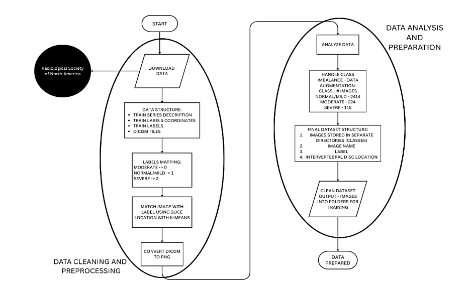
This image has an empty alt attribute; its file name is image-102.png

Figure 1 – Data Cleaning and Processing Workflow

4.1. DATASET (CONVERT THE DATASET CONTENT INTO A FLOWCHART TO OPTIMIZE THE READING)

The dataset, graciously provided by the Radiological Society of North America, comprises high-resolution lumbar spine MRI scans acquired in DICOM (Digital Imaging and Communications in Medicine) format. This format not only ensures the preservation of detailed image metadata and acquisition parameters but also facilitates standardized, reproducible analyses across diverse clinical imaging systems. The dataset is further enriched with expert-annotated severity ratings for five distinct degenerative conditions, systematically documented across the intervertebral disc levels ranging from L1/L2 to L5/S1. These annotations serve as critical ground-truth labels, enabling rigorous evaluation of computational models in discerning subtle gradations of degenerative changes. Moreover, the comprehensive nature of this dataset underpins its utility as a robust benchmark for developing advanced deep learning algorithms aimed at automated diagnostic classification and segmentation in computational radiology.

4.1.1. RAW DATA STRUCTURE

The data utilized in this study was initially provided in multiple CSV files and DICOM images, which required significant preprocessing to organize the data for deep learning model training. The key raw files included:

1. Train Series Description CSV
This file covers essential metadata about each MRI scan, detailing the scan type and series ID for every patient. This information is crucial for understanding the imaging sequences used and for filtering the relevant slices needed for classification tasks.

2. Train Labels Coordinates CSV
This file provides bounding box coordinates that pinpoint the exact regions of interest (ROIs) for each degenerative condition. It plays a vital role in segmentation tasks, especially when future research may focus on isolating specific areas for detailed analysis.

3. Train Labels CSV
This file contains the condition labels for each MRI scan, associating each patient and series ID with their corresponding classification (Normal/Mild, Moderate, Severe). These labels are used for training the model to distinguish between different levels of degeneration.

4. DICOM Files
These files contain the actual MRI scan images in DICOM format, which include detailed 3D volumetric data of the lumbar spine regions. These images were parsed and converted into a suitable format for deep learning processing to ensure compatibility with the model architecture.

The preprocessing steps involved organizing these files to ensure consistency and structure, enabling effective training of deep learning models.

4.1.2. DATA CLEANING AND PREPROCESSING

To prepare the dataset for training, several critical preprocessing steps were performed to ensure its suitability for deep learning models. The severity labels (Normal/Mild, Moderate, Severe) were mapped to numerical values, facilitating efficient classification. Since DICOM files lacked explicit labels, metadata was used to align MRI scan slices with the corresponding condition labels. To further streamline the process, K-Means clustering was applied to group MRI slices based on spinal levels, ensuring proper alignment with condition labels. Additionally, DICOM images were converted to PNG format, with grayscale normalization applied to standardize image quality. Finally, due to class imbalance in the dataset, data augmentation techniques were employed to enhance underrepresented classes, improving the model’s generalization. These preprocessing steps ensured that the dataset was properly structured for effective training and accurate predictions.

• Mapping Categorical Values to Numerical Labels
The severity labels (Normal/Mild, Moderate, Severe) were mapped to integer values as we show on Table 1:

Table 1 – Mapping relationships between Categorical Value and Numerical Value.

Severity Labels | Mapping Value
Moderate | 0
Normal/Mild | 1
Severe | 2

◦ This transformation ensured compatibility with neural network’s loss function and allowed for efficient classification.

• Handling Class Imbalance

◦ The dataset presented a class imbalance issue, where the “Normal/Mild” class had a substantially higher number of samples compared to the “Moderate” and “Severe” conditions. This imbalance can cause issues during model training, as the model may become biased towards the more frequent class (Normal/Mild) and perform poorly on the less represented classes (Moderate and Severe). As shown in Table 2, we do not have a balanced number of images per class, and there is a need for augmentation to solve this issue. Addressing this imbalance is essential to ensure that the model learns to classify all conditions accurately. Methods such as data augmentation or resampling are typically applied to balance the dataset, helping the model generalize better across all categories.

Table 2 – Amount of images pre-augmentation per class

Class | Number of Images
Normal/Mild | 2414
Moderate | 224
Severe | 115

◦ To tackle the issue of class imbalance, data augmentation techniques were employed to artificially increase the representation of the underrepresented classes, namely “Moderate” and “Severe” conditions. This process involves generating new, synthetic samples from the existing data through various transformations such as rotation, flipping, scaling, and cropping. By applying these techniques, the model was exposed to a more balanced dataset, with a greater variety of images for the underrepresented classes. This approach helps the model learn better generalization and improves its ability to classify less frequent classes accurately, ultimately enhancing the performance of the model on real-world data where such imbalances may exist.

4.1.3. FINAL PROCESSED DATASET

After the data cleaning and augmentation process, the final dataset was organized in the following way:

1. Images stored in separate directories based on severity class (Normal_Mild, Moderate, Severe):
The images were categorized and stored in distinct folders based on the severity of the condition they represent (Normal/Mild, Moderate, or Severe). This organization ensures that each class is easily identifiable and accessible during model training.

2. Label annotations mapped numerically to facilitate training:
To make the labels compatible with the deep learning model, the severity categories were converted into numerical values. For example, “Normal/Mild” may have been assigned the value 1, “Moderate” assigned 0, and “Severe” assigned 2. This numerical encoding allows the model to interpret and process the labels during training.

3. Intervertebral disc levels correctly assigned using slice location clustering:
MRI images contain multiple slices corresponding to different spinal levels (such as L1/L2, L2/L3). Using a technique called slice location clustering, the slices were correctly grouped by their anatomical location. This ensured that each MRI slice was assigned to its correct intervertebral disc level, providing the necessary anatomical context for training.

4. Balanced class distribution achieved through augmentation techniques:
Initially, the dataset was imbalanced, with a significantly higher number of images in the “Normal/Mild” class compared to the “Moderate” and “Severe” classes. To address this, data augmentation techniques (such as rotations, zooms, etc.) were used to artificially increase the number of images in the underrepresented classes. This helped balance the class distribution, ensuring the model was not biased toward the more frequent class.

4.2. DATA ANALYSIS

The initial data analysis began by parsing the DICOM files to extract key metadata, including patient ID, series ID, and slice location. Series ID tells you what type of MRI scan was performed. Different series IDs correspond to different MRI imaging methods (like T1-weighted, T2-weighted, or diffusion-weighted), each designed to show certain tissues or conditions more clearly. Slice location tells you exactly where within the body an MRI image was taken. It represents the specific height or position of that image slice. The slice location data played a crucial role in organizing the images according to specific intervertebral disc levels. To achieve this, an unsupervised K-Means clustering algorithm was applied to group the slices, ensuring proper alignment of images with their respective labels.

To address the class imbalance, an examination of the distribution of severity labels revealed a significant overrepresentation of the Normal/Mild class. As a result, data augmentation techniques were implemented to balance the class distribution and ensure more equitable representation across all severity levels. As we can see in Table 3, our data is now balanced and ready for the next steps of the process.

Table 3 – Number of Images post-augmentation per class

Class | Number of Images
Normal/Mild | 2146
Moderate | 2148
Severe | 2164

4.3. DATA AUGMENTATION

Data augmentation was implemented to enhance model generalization and mitigate overfitting. To make sure that the data augmentation does not give us any problems on the construction of model, we created a 1:1 ratio of augmenting data on the Normal/Mild class, and we created the necessary images to balance the data. In the training, only data that has been augmented was used, not original images. The ImageDataGenerator function from TensorFlow was utilized with the following parameters:

• Width Shift Range: 0.1
• Height Shift Range: 0.1
• Zoom Range: 0.1
• Horizontal Flip: True
• Fill Mode: ‘nearest’

These augmentations effectively increased the representation of underrepresented classes, resulting in a more balanced dataset. Figure 2 shows an example of 4 images of the training dataset, which has been augmented. On the top of the image, it is printed the class that they belong to, following the structure of Table 1. Corresponding 0:Moderate, 1:Normal/Mild, 2:Severe.

Figure 2 – Sample of images with their assigned class after augmentation

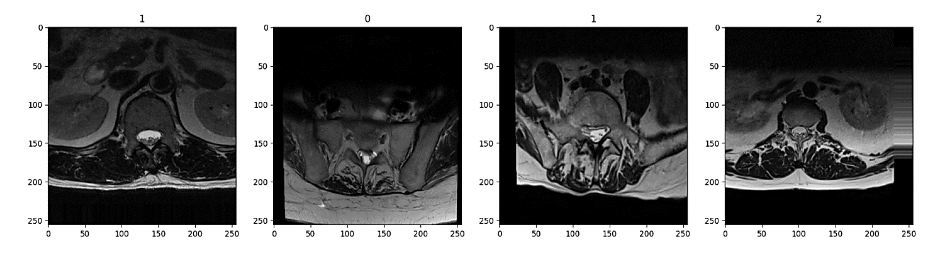
This image has an empty alt attribute; its file name is image-103.png

Figure 2 shows four sample images after augmentation, each labeled with its assigned class at the top. From left to right, the first image (class 2) appears with minimal tilt. The second image (class 1) is slightly rotated to the right, noticeable in the shift of the spinal structures and the darker region on one side. The third image (also class 1) similarly has a slight rightward tilt, although less pronounced. Finally, the fourth image (class 1) is tilted to the left, and its lower portion appears deeper in the scan, giving a more pronounced sense of depth compared to the others. (one image for pre-augmentation and another post-augmentation)

4.4. RESEARCH MODEL: LAYERS AND ARCHITECTURE

A convolutional neural network (CNN) was selected to develop a predictive model for classifying images into severity categories due to its proven efficacy in processing grid-structured, image-based data. CNNs constitute a deep learning architecture designed explicitly for feature extraction from images, identifying

characteristics such as edges, textures, and intricate spatial patterns through sequential convolution and pooling operations.

TensorFlow and Keras were employed for the construction and training of the CNN model. TensorFlow, an open-source machine learning framework developed by Google, provides robust computational resources particularly suited for deep neural network computations. Complementing TensorFlow, Keras serves as a high-level, user-friendly API facilitating efficient development, experimentation, and refinement of neural network architectures. The combination of these frameworks considerably streamlined the implementation, enabling efficient construction of convolutional and pooling layers, alongside other essential components. Consequently, this methodology facilitated the effective construction, training, and integration of the CNN model, achieving accurate real-time classification of image severity.

This model has been built using the “Sequential” function of the Keras API integration. This function allows us to build a CNN model that will be trained on images, that later on will help us predict patients’ conditions. In the design of this model, we have developed 5 convolution blocks that will allow us to determine and examine the features of the MRIs, to be able to predict with a higher accuracy, as shown in Figure 3. Each block contains different types of layers, in which each of those layers have a specific purpose. The layers in the convolutional blocks are the following:

1. Input Layer:
Processes 256×256 RGB images. This resolution and the RGB color space were strategically chosen to balance detailed feature capture with computational efficiency. The specified image size ensures sufficient spatial detail to identify intricate features without significantly increasing computational demands. Employing the RGB model’s three-channel color representation enhances the network’s capacity to discern subtle color-based details crucial for accurate image classification.

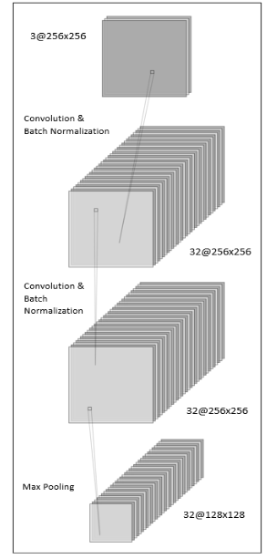
This image has an empty alt attribute; its file name is image-104.png

Figure 3 – Convolutional Block Diagram Example

2. Convolutional Layers:
Each convolutional block incorporates two convolutional layers with filter sizes progressively increasing from 32 to 512, employing ReLU activation functions. These layers apply filters across images to detect and extract essential features, such as edges and textures, generating foundational feature maps for subsequent analysis.

3. Batch Normalization Layers:
Integrated immediately after each convolutional layer to stabilize and expedite the training process. These layers normalize outputs from preceding layers, reducing internal covariate shifts and ensuring consistent feature scaling.

4. Max Pooling Layers:
Positioned after each pair of convolutional layers to decrease the spatial dimensions of feature maps by retaining the maximum value from defined regions. This approach conserves critical features while reducing computational complexity.

5. Dropout Layers:
Convert the multi-dimensional feature maps from previous layers into a one-dimensional vector, making the data suitable for input into fully connected layers.

6. Flatten Layer:
Functions as a fully connected layer where every neuron is connected to every neuron in the previous layer, combining the extracted features to perform classification, such as assigning the image to a specific severity class.

7. Dense Layer:
Operates as a fully connected layer, linking every neuron to those in preceding layers. This layer synthesizes the extracted features to facilitate classification tasks, such as assigning each image to its corresponding severity category.

The detailed composition of these convolutional blocks, as illustrated in Figure 3, provides a systematic approach to feature extraction and classification, contributing significantly to the predictive performance of the CNN model.

After the convolutional blocks extract features, the model transitions to fully connected layers to consolidate this information for classification. This representation is also visually explained on Figure 4. In essence:

• Feature Integration: The Flatten layer converts the multi-dimensional feature maps into a vector, which is then processed by two Dense layers (with 512 and 256 neurons, respectively) using ReLU activation. Batch normalization and dropout (50%) are applied after each dense layer to stabilize training and reduce overfitting.

• Output & Compilation: A final Dense layer with 3 neurons and softmax activation produces class probabilities, and the model is compiled with the Adam optimizer and sparse categorical crossentropy loss, ensuring effective multi-class classification.

The model was compiled using the Adam optimizer, which adjusts learning rates during training to help the model converge efficiently, alongside the sparse categorical crossentropy loss function, which is ideal for multi-class classification tasks. An EarlyStopping callback was also implemented to monitor validation loss, stopping training if no improvement occurs for 5 consecutive epochs. This prevents overfitting and excessive training, while restoring the best weights achieved during the training process to ensure optimal performance.

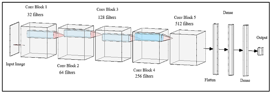
This image has an empty alt attribute; its file name is image-106.png

Figure 4 – Model Architecture Diagram

5. Results

The Sequential model was initially configured to undergo training for 25 epochs. However, an early stopping mechanism was implemented as a regularization strategy to prevent overfitting. Early stopping monitors the model’s performance on a validation set and halts training once further epochs no longer yield meaningful improvements in generalization. This mechanism, underpinned by the dynamics of gradient descent and the structure of the loss landscape, effectively controls model complexity and balances the bias-variance trade-off. In our experiments, although the training was scheduled for 25 epochs, the process was terminated at the 16th epoch because the validation performance plateaued, indicating that additional training would have likely led to overfitting through the memorization of noise in the training dataset.

The training and validation accuracy illustrated in Figure 5 as well as the loss metrics shown in Figure 6 were carefully monitored throughout the process to determine the optimal stopping point. It is important to note that the entire training process was executed in a CPU-only environment using Jupyter Notebooks, without the benefit of GPU acceleration. As a consequence, the overall training duration extended to approximately two hours, reflecting the increased computational time required when running on CPU resources. This setup, while less time-efficient than GPU-based alternatives, provided a robust platform fiterative model development and real-time monitoring of training dynamics.

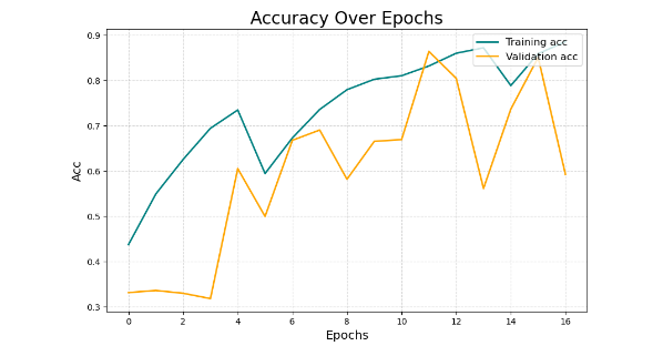
This image has an empty alt attribute; its file name is image-107.png

Figure 5 – Depicts the training and validation accuracy over the epochs (Acc stands for Accuracy in this graph)

As illustrated in Figure 6, the training accuracy shows a steady increase, while the validation accuracy demonstrates an initial rise followed by stabilization, indicating effective learning and generalization.

Figure 7 shows a consistent decrease in both training and validation loss, further confirming the model’s learning efficacy.

From the plotted accuracy and loss curves on Figures 11 and 12, it is evident that the validation loss starts to rise sharply around epoch 12, while the training loss continues to decline. This divergence signals the onset of overfitting: the model begins to memorize training examples rather than learning transferable patterns. The early stopping callback, configured with a patience of 5 epochs, automatically halts training at this point because the validation performance fails to improve for five consecutive epochs. Although training could continue up to epoch 25, the trend suggests that the validation loss would not improve any more, remaining constant. Beyond epoch 12, the model would start to memorize the training data and would generalize poorly, since the training will continue to improve, and the validation will remain constant.

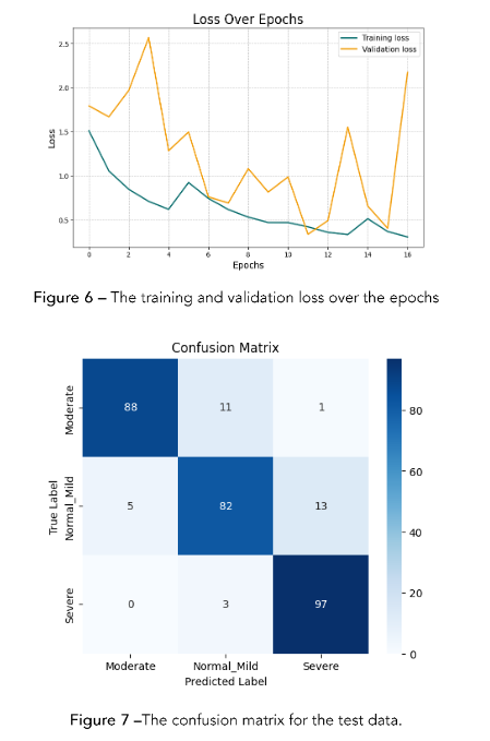
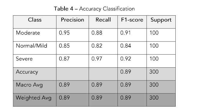
This image has an empty alt attribute; its file name is image-108.png

Figure 7 – The confusion matrix for the test data.

6. Confusion Matrix

To evaluate the model’s performance, we saved 300 images from the non-augmented dataset. We used that dataset (100 normal, 100 moderate, and 100 severe) to evaluate the model’s performance on unseen data. The model’s performance was evaluated using a confusion matrix, which is presented in Figure 8, precision, recall, and F1-score metrics on the test dataset.

In Figure 7, the diagonal elements represent the correctly classified instances for each class, while off-diagonal elements indicate misclassifications.

The confusion matrix illustrates how the model performs across the three classes—Moderate, Normal/Mild, and Severe—by comparing actual labels (rows) against predicted labels (columns). For instance, of the 100 “Moderate” images, the model correctly classifies 88, while misclassifying 11 as “Normal/Mild” and 1 as “Severe.” This outcome corresponds to a recall of 0.88 for the Moderate class, signifying that 88% of actual Moderate samples are correctly identified. Similarly, the model achieves its highest recall (0.97) on the Severe class, indicating that 97 out of 100 Severe images are accurately detected. In contrast, the Normal/Mild class has a

recall of 0.82, reflecting that 18% of those images are misclassified as either Moderate or Severe.

Precision captures how often a predicted label is correct relative to all predictions made for that label. The Moderate class achieves the highest precision (0.95), meaning that when the model predicts “Moderate,” it is correct 95% of the time. Meanwhile, Severe has a precision of 0.87, suggesting a moderate rate of false positives for that class, and Normal/Mild’s precision stands at 0.85. The F1-score, which harmonically balances precision and recall, further highlights these differences: the Severe class exhibits the highest F1-score (0.92), while Normal/Mild has the lowest (0.84). Overall, the model attains an accuracy of 89%, correctly classifying 267 out of 300 images. Although these results demonstrate robust performance, the confusion matrix helps pinpoint specific misclassification patterns—particularly between Moderate and Normal/Mild—indicating areas where further refinement may enhance the model’s diagnostic accuracy.

The model’s performance was evaluated using precision, recall, and F1-score on the test dataset. The updated classification metrics are as follows:

• Moderate: Precision: 0.95, Recall: 0.88, F1-score: 0.91
• Normal/Mild: Precision: 0.85, Recall: 0.82, F1-score: 0.84
• Severe: Precision: 0.87, Recall: 0.97, F1-score: 0.92

The overall accuracy achieved was 89%, and the metrics we mentioned above are shown in Table 4.

This image has an empty alt attribute; its file name is image-109.png

Table 4 presents the classification performance metrics of the trained convolutional neural network (CNN) model on the test dataset. It includes precision, recall, and F1-score for each class (Moderate, Normal/Mild, and Severe) along with overall accuracy and average performance scores.

The model’s overall accuracy of 89% indicates that it correctly classifies 89% of all tested samples across all classes, offering a broad measure of its predictive capability. However, the notably high recall (0.97) on the Severe condition is particularly important, as it minimizes the likelihood of missing critical cases that demand immediate attention.

7. Discussion

The promising results of this research highlight the potential of deep learning in automating the classification of Spinal Canal Stenosis (SCS) from axial T2-weighted MRI scans. Achieving a high accuracy and remarkable recall for the Severe category suggests that CNNs can effectively identify subtle imaging patterns that may be overlooked or inconsistently interpreted by human observers.

These outcomes are particularly significant given the clinical importance of accurately distinguishing between Normal/Mild, Moderate, and Severe

cases of SCS. Early identification of severe stenosis is critical, as it often necessitates surgical intervention or targeted therapeutic planning. By reducing the risk of misclassification, this model can serve as a valued second opinion for radiologists and spine specialists, potentially improving diagnostic confidence and consistency.

Techniques such as DICOM-to-PNG conversion, K-Means clustering for selecting the most relevant slices, and targeted data augmentation to address class imbalance ensured that the model received high-quality and diverse input data. This emphasizes the role of careful data preparation in medical imaging applications, where input variability and class imbalance are common challenges.

However, despite these strengths, there are limitations that should be acknowledged. The model was trained exclusively on axial T2-weighted scans, which, while informative, may not capture the full anatomical context that sagittal views or multimodal inputs could provide. Additionally, while the recall for Severe cases is high, further evaluation is needed to ensure consistent performance across all severity levels, especially in real-world clinical settings with varied imaging protocols.

8. Conclusion

This study successfully developed a CNN-based model for classifying lumbar spinal canal stenosis using MRI scans, highlighting the critical importance of detailed feature extraction in medical imaging analysis. A key realization from this research is that meticulous feature extraction, facilitated through additional convolutional layers and careful filtering techniques, significantly contributes to the model’s diagnostic performance. By implementing rigorous data preprocessing, effective augmentation strategies to address class imbalance, and an optimized deep learning architecture comprising five convolutional blocks, the model achieved an overall classification accuracy of 89%, particularly notable was the model’s exceptionally high recall of 97% in the Severe class, emphasizing the value of precise feature extraction in accurately diagnosing critical cases requiring urgent clinical intervention.

Although the findings illustrate significant progress, there is still room for further improvement by expanding the dataset to include additional MRI scans from diverse clinical sources, thereby enhancing the model’s generalization and robustness. Future research exploring transformer-based architectures, specifically Vision Transformers (ViTs), could further capitalize on the detailed features present in medical images by capturing long-range dependencies, potentially yielding even greater accuracy. Additionally, incorporating clinical metadata into multimodal learning frameworks could further augment classification performance and diagnostic accuracy, underscoring the role comprehensive feature integration plays in advancing medical imaging diagnostics.

Lastly, practical deployment considerations, including interpretability, reliability, and computational efficiency, must be prioritized to ensure successful clinical adoption. Collectively, this research contributes significantly to the advancement of automated medical imaging analysis by underscoring the importance of sophisticated feature extraction techniques, detailed insights into model training dynamics, and the integration of advanced architectures and multimodal strategies within clinical workflows.

Model’s overall accuracy of 89% indicates that it correctly classifies 89% of all tested samples across all classes, offering a broad measure of its predictive capability. However, the notably high recall (0.97) on the Severe condition is particularly important, as it minimizes the likelihood of missing critical cases that demand immediate attention.

7.1. Final Remarks

This research contributes to the growing field of AI-driven medical diagnostics, providing a structured approach to deep learning-based spine imaging analysis. Further research into more sophisticated

References

Buda, Mateusz, Atsuto Maki, and Maciej A. Mazurowski. 2018. “A systematic study of the class imbalance problem in convolutional neural networks.” Neural Networks 106: 249–259.
https://doi.org/10.1016/j.neunet.2018.07.011

Chmelik, Jiri, Roman Jakubicek, Petr Walek, Jiri Jan, Petr Ourednicek, Lukas Lambert, Elena Amadori, and Giampaolo Gavelli. 2018. “Deep convolutional neural network-based segmentation and classification of difficult to define metastatic spinal lesions in 3D CT data.” Medical Image Analysis 49: 76–88.
https://doi.org/10.1016/j.media.2018.07.008

Farooq, Muhammad, and Abdul Hafeez. 2020. “Covid-ResNet: A deep learning framework for screening of COVID-19 from radiographs.” arXiv preprint arXiv:2003.14395.

Li, Hao, Gopi Krishnan Rajbahadur, Dayi Lin, Cor-Paul Bezemer, and Zhen Ming Jiang. 2024. “Keeping Deep Learning Models in Check: A History-Based Approach to Mitigate Overfitting.” IEEE Access 12: 70676–70689.
https://doi.org/10.1109/ACCESS.2024.3402543

Lim, Desmond Shi, Andrew Makmur, Lei Zhu, Wenqiao Zhang, Amanda J. Cheng, David Soon Sia, Sterling Ellis Eide, et al. 2022. “Improved productivity using deep learning–assisted reporting for lumbar spine MRI.” Radiology 305 (1): 160–66. https://doi.org/10.1148/radiol.220076

Munadi, Khairul, Kahlil Muchtar, Novi Maulina, and Biswajeet Pradhan. 2020. “Image enhancement for tuberculosis detection using deep learning.” IEEE Access 8: 217897–907.
https://doi.org/10.1109/ACCESS.2020.3041867

Neubert, A., J. Fripp, C. Engstrom, R. Schwarz, L. Lauer, O. Salvado, and S. Crozier. 2012. “Automated detection, 3D segmentation and analysis of high resolution spine MR images using statistical shape models.” Physics in Medicine and Biology 57 (24): 8357–76. https://doi.org/10.1088/0031-9155/57/24/8357

Ng, H.P., S.H. Ong, K.W.C. Foong, P.S. Goh, and W.L. Nowinski. 2006. “Medical Image Segmentation Using K-Means Clustering and Improved Watershed Algorithm.” In Proceedings of the IEEE International Conference on Image Processing, 611-614. https://doi.org/10.1109/ICIP.2006.312517

Özkaraca, Osman, Okan İhsan Bağrıaçık, Hüseyin Gürüler, Faheem Khan, Jamil Hussain, Jawad Khan, and Umm e Laila. 2023. “Multiple brain tumor classification with dense CNN architecture using brain MRI images.” Life 13 (2): 349. https://doi.org/10.3390/life13020349

Processing of MR images for efficient quantitative image analysis using deep learning techniques.” In Proceedings of the 2017 International Conference on Recent Advances in Electronics and Communication Technology (ICRAECT), 191–95. https://doi.org/10.1109/icraect.2017.43

Ruiz-España, Silvia, Estanislao Arana, and David Moratal. 2015. “Semiautomatic computer-aided classification of degenerative lumbar spine disease in magnetic resonance imaging.” Computers in Biology and Medicine 62: 196–205. https://doi.org/10.1016/j.compbiomed.2015.04.028

Scannell, Cian M., Mitko Veta, Adriana D.M. Villa, Eva C. Sammut, Jack Lee, Marcel Breeuwer, and Amedeo Chiribiri. 2020. “Deep-Learning-Based Preprocessing for Quantitative Myocardial Perfusion MRI.” Journal of Magnetic Resonance Imaging 51: 1689–1696. https://doi.org/10.1002/jmri.26983

Seo, Hyunseok, Lequan Yu, Hongyi Ren, Xiaomeng Li, Liyue Shen, and Lei Xing. 2021. “Deep neural network with consistency regularization of multi-output channels for improved tumor detection and delineation.” IEEE Transactions on Medical Imaging 40 (12): 3369–78. https://doi.org/10.1109/tmi.2021.3084748

Villmann, Thomas, Marika Kaden, Mandy Lange, and Paul Stürmer. 2014. “Precision-Recall-Optimization in Learning Vector Quantization Classifiers for Improved Medical Classification Systems.” In Proceedings of the 2014 International Joint Conference on Neural Networks (IJCNN), 195–202. https://doi.org/10.1109/IJCNN.2014.6889664

Suzuki, Hisataka, Terufumi Kokabu, Katsuhisa Yamada, Yoko Ishikawa, Akito Yabu, Yasushi Yanagihashi, Takahiko Hyakumachi, et al. 2024. “Deep Learning-Based Detection of Lumbar Spinal Canal Stenosis Using Convolutional Neural Networks.” The Spine Journal 24 (11): 2086–2101. https://doi.org/10.1016/j.spinee.2024.06.009.

Zhou, Zhiyi, Shenjun Wang, Shujun Zhang, Xiang Pan, Haoxia Yang, Yin Zhuang, and Zhengfeng Lu. 2024. “Deep Learning-Based Spinal Canal Segmentation of Computed Tomography Image for Disease Diagnosis: A Proposed System for Spinal Stenosis Diagnosis.” Medicine 103 (18): e37943. https://doi.org/10.1097/MD.0000000000037943.

Yoo, Hyunsuk, Roh-Eul Yoo, Seung Hong Choi, Inpyeong Hwang, Ji Ye Lee, June Young Seo, Seok Young Koh, Kyu Sung Choi, Koung Mi Kang, and Tae Jin Yun. 2023. “Deep Learning-Based Reconstruction for Acceleration of Lumbar Spine MRI: A Prospective Comparison with Standard MRI.” European Radiology 33 (12): 8656–68.
https://doi.org/10.1007/s00330-023-09918-0.

Jeon, Yejin, Bo Ram Kim, Hyoung In Choi, Eugene Lee, Da-Wit Kim, Boorym Choi, and Joon Woo Lee. 2025. “Feasibility of Deep Learning Algorithm in Diagnosing Lumbar Central Canal Stenosis Using Abdominal CT.” Skeletal Radiology 54 (5): 947–57. https://doi.org/10.1007/s00256-024-04796-z.

Hokamura, Masamichi, Takeshi Nakaura, Naofumi Yoshida, Hiroyuki Uetani, Kaori Shiraishi, Naoki Kobayashi, Kensei Matsuo, et al. 2024. “Super-Resolution Deep Learning Reconstruction Approach for Enhanced Visualization in Lumbar Spine MR Bone Imaging.” European Journal of Radiology 178. https://doi.org/10.1016/j.ejrad.2024.111587.