Gaussian Graphical Model Estimations in Multivariate Linear Regression: A method and applications in omics studies

Irene SuiLan Zeng^1,2, Thomas Lumley¹

1. University of Auckland, Department of Statistics ;  Auckland University of Technology, School of Clinical Science, Biostatistics
2. University of Auckland, Department of Statistics

OPEN ACCESS

PUBLISHED: 31 December 2024

CITATION: ZENG, Irene SuiLan; LUMLEY, Thomas. Gaussian Graphical Model Estimations in Multivariate Linear Regression: A method and applications in omics studies. Medical Research Archives. Available at: <https://esmed.org/MRA/mra/article/view/6088>.

COPYRIGHT: © 2025 European Society of Medicine. This is an open-access article distributed under the terms of the Creative Commons Attribution License, which permits unrestricted use, distribution, and reproduction in any medium, provided the original author and source are credited.

DOI: https://doi.org/10.18103/mra.v12i12.6088

ISSN 2375-1924

Abstract

Introduction: Regression models for high-dimensional multivariate data curated from high throughput biological assays in omics, brain networks, medical imaging, and psychometric instruments contain network features. Multivariate linear regression is a standard model that fits these data as response variables and the participant characteristics as explanatory variables. More often, the number of variates of the response variables (𝑝) is larger than the number of observations (𝑛). To solve these problems, a structured covariance model is necessary to maintain the network feature of the response data, and sparsity induction will be advancing to reduce the number of unknown parameters in the large variance-covariance matrix. Method: This study investigated an approach to solving multivariate linear regression for multivariate-normal distributed response variables using a sparsity-induced latent precision matrix. The multivariate linear regression coefficients were derived from an algorithm that estimated the precision matrix as a plug-in parameter using different Gaussian Graphical Models. The developed Bioconductor tool “sparsenetgls” based on this algorithm was applied to case studies of real omics datasets. Data simulations were also used to compare different Gaussian Graphical Models estimation methods in multivariate linear regression. Results: The GGM multivariate linear regression (GGM-MLS) advances the multivariate regression. In the scenario when the number of observations is smaller than the number of response variates (𝑛 < 𝑝), GGM-MLS tackles this challenge using sparsity induction in the covariance matrix. Analytical proof suggests that the estimation of the response variable’s precision matrix and the regression coefficient of GGM-MLS are two independent processes. Simulation studies and case studies also consistently suggested that the regression coefficient estimates of GGM-MLS are similar to the estimates using linear mixed regression with only the variance terms in the covariance matrix. Furthermore, GGM-MLS method reduces the variance (standard errors) of the regression coefficients in both 𝑛 < 𝑝 and 𝑛 > 𝑝 scenarios.

Keywords: GGM in multivariate linear regression, network outcome responses, omics data analysis, sparsity induction in multivariate linear regression.

1. Introduction

In regression models for Gaussian multivariate data curated from high-throughput (e.g., “omics”) and other biomedical, imaging, and psychometrics instruments with high dimensionality, the response (outcome) variables have their latent graph structures presented by the precision matrix. The graph structure could be interpreted by the network of these response variables’ related fields (e.g., expressions of genes and abundance of proteins/metabolites from their biological pathways, brain network, EEG, MRI, and psychometrics measurements of different functionalities). The common question is to identify and estimate the impacts of the predictors on these responses (outcomes) variables presented in the study. The predictors could include experimental design, clinical design parameters, and other exposure variables. However, the challenge in the high-throughput omics and other high-dimensional outcome data is that the number of response variables is much larger than the number of observations. Although dimensional reduction in the response variables could be considered, the interpretation in its context without further validation could be complex in the multivariate linear regression.

Our solution to the problem is to use a graphical model to induce the sparsity in the precision matrix and its variance-covariance matrix of the response variables to achieve better estimation in the multivariate regression while keeping the dimension of the response variable or the subset of the dimensions (e.g., responses in a biological pathway). We suggest a covariance selection method utilizing the graph structure—the adjacency matrix 𝐴 for the underlying graph of the precision matrix. This method considers the precision matrix of the response variables as a nuisance plug-in estimator from GGM in deriving the fixed effect regression coefficients of the multivariate linear regression. We aim to improve the fixed effect coefficients utilizing the graph information related to the precision matrix of the response variables.

1.1 MULTIVARIATE MODELS AND MULTILEVEL MODELS

Goldstein introduced a multilevel model that constructs the multivariate Gaussian distributed response variable as a special case of the two-level model. Under this multilevel model, the response variable constituted hierarchical levels, with first level (level one) units representing the primary sampling units (PSU). These could be, for example, omics platforms, trial participants, hospital wards, and clinical centres. The second level comprised the measure of each variate of the response, such as the protein quantity constructed by multiple-ions abundance, expression of multiple genes from the same biological network, and brain network signatures measured from the same cluster. The identification vector, representing the first level unit (e.g., protein, trial participant) of the multivariate distributed response, is included in the model as a random effect. To estimate the variance-covariance matrix of the random effect, Pinheiro and Bates used a relative precision factor Δ as the function of the precision matrix Σ^-1 of the random effect: 𝜎²Σ^-1 = ΔΔ^T, One simple form of the Δ, is the relative precision ratio (a scalar) between the variance of unexplained random errors and the variance between 𝑝 groups in the estimation √𝜎² /𝜎_𝑝². Standard errors of fixed effect regression coefficients β are estimated from the variance 𝜎²[∑ 𝑋_𝑖 M^T_𝑖=1 Σ_𝑖^-1𝑋_𝑖]^-1, where 𝑀 represents the number of multidimensional response variables; 𝑋_𝑖, is the 𝑖^th data matrix and Σ_𝑖^-1 its inverse variance-covariance matrix. The approximated variance-covariance matrix Σ of the multiple responses is estimated using the relative precision factor Δ. Goldstein suggested an alternative approach, using the Jackknife method to estimate the standard error. Few methods use the Gaussian Graphical Model (GGM) to estimate the precision matrix or the variance-covariance matrix within multilevel and mixed-effect regressions.

1.2 METHODS AND ALGORITHMS USED IN GAUSSIAN GRAPHICAL MODELS (GGM)

In the large-dimensional data problem, sparse induction is a general approach for estimating the precision matrix. There are two streams of GGM estimation for the sparse precision or variance-covariance matrix. Yuan and Lin, Friedman, Hastie, Simon and Tibshiran, Friedman, Hastie and Tibshirani used the 𝑙₁ penalized Maximum likelihood of the precision matrix and utilized Maxdet and blockwise-coordinate-descent algorithm, respectively, to estimate the graph structure under positive-definite constraints. Meinshausen and Buhlmann, Friedman, Hastie and Tibshirani, and Peng, Wang, Zhou and Zhu used the 𝑙₁ penalized linear least-squares regressions among response variables to approximate the covariance and partial correlation coefficient matrix. Meinshausen and Buhlmann also included neighbourhood selections in the penalized linear regression. The maximum likelihood method estimates all unknown edges of the graph simultaneously. The linear regression method assumes conditional dependence among the response variables and regresses each data matrix’s column on the rest of the other columns. It has been proved that the linear regression approximation is the second-order Taylor series approximation of the maximum likelihood solution.

In addition to these GGM methods, motivated by the covariate effects arising from the genetic genomic problem, Cai, Li, Liu, and Xie included covariates in the estimation of the response variables’ sparse precision matrix using a two-stage constrained minimization. A recent development in a similar stream modelled the covariate effects on the precision matrix of the response variables and a 2-step selection of the covariance term in the block diagonal covariance matrix. In the opposite direction of solving the covariate-effect problem, we utilized the graphical structure of the response variables to improve the estimation of regression coefficients in multivariate regression. We studied different GGM estimation methods to derive the graph structure of the response variables and, based on the estimated graph structure, to derive the fixed regression coefficients and their variance in MLS. This solution can be applied to estimate the attribute and treatment effect and identify significant exposure factors on a group of genes’ expressions, proteins’ abundances, brain connectivity network fMRI measures, and other high-dimensional outcome responses.

2. Method

2.1 CONSTRUCT A MULTIVARIATE REGRESSION MODEL VIA A TWO-LEVEL MODEL WITH PRECISION AND VARIANCE-COVARIANCE MATRIX

A multivariate regression model with only fixed effects can be expressed as a two-level mixed-effect model with one random effect, an identification variable, for each variate of the 𝑝-dimensional multivariate response. The configurations of this two-level model, when the response is multivariate normal, are as follows: 𝒚 = 𝑋^*𝛽 + 𝑍𝝁 + 𝒆; 𝒖 ∼ 𝑁(0, Σ); 𝒆 ∼ N(0, δ²) (1) where, 𝒚 = (𝒚₁, 𝒚₂, … 𝒚_𝑛)^T, 𝑋 = {𝟏, 𝑥_𝑖𝑗}, 𝑖 = 1 … 𝑛; 𝑗 = 1 … 𝑝 𝑋^* = (𝑋, … 𝑋)^T(𝑞+1)×(𝑛^*𝑝) 𝒖 = (𝑢₁, … 𝑢_𝑗 … 𝑢_𝑝), 𝑍 = {𝒛_{1</sub} … 𝒛𝑗 … 𝒛𝑝}^T, 𝒛𝑗 = {𝟎 𝟏 Let 𝐲 be the stacked vectorized format of the response variable matrix 𝑌𝑛×𝑝, where 𝑝 equals the number of dimensions of the response variable 𝑌, 𝑛 is the number of subjects. {𝒚𝑖} is a 𝑝-element column-vector, where 𝒚𝑖 = (𝑦𝑖,1, … 𝑦𝑖,𝑝)^T, 𝑖 = 1 … 𝑛. 𝑋 is the design matrix of 𝑞 fixed effects, and 𝑋^* is the (𝑛𝑝) × 𝑞 matrix stacking 𝑋 for 𝑝 times. 𝑍 represents the (𝑛𝑝) × 1 identification matrix of the p-dimensional response, Σ is the variance-covariance matrix of 𝑌𝑛×𝑝. The profile log-likelihood function of (𝛃,Ω) is 𝐿(𝛃,Ω) = − log|Ω^-1| − 𝑡𝑟(ΩS), where Ω = Σ^-1 is the precision matrix of 𝑌. Substituting the sample variance-covariance matrix 𝑆 = (𝑌 − 𝑋β)^T(𝑌 − 𝑋β), into the profile log-likelihood thus is 𝐿(β,Ω) = − log|Ω^-1| − (𝑌 − 𝑋β)^TΩ^T(𝑌 − 𝑋β) (2). Let the estimation function w.r.t β derived from the derivative of (2) be: 𝜕𝐿/𝜕𝛽|β,Ω = 𝜓β,Ω = (−𝑋^T)Ω(𝑌 − 𝑋β), the next derivative w.r.t β is 𝜕𝜓/𝜕𝛽|β,Ω = 𝜓̇β,Ω = 𝑉β,Ω = (𝑋^TΩ𝑋). In the multilevel framework, the estimation function and its derivative function w.r.t 𝛃 can be notated using the vector 𝒚 and stacked matrix 𝑋^* and Ω^*: 𝜓β,Ω* = (−𝑋^*T)Ω^*(𝒚 − 𝑋^*β); 𝜓̇β,Ω = 𝑉β,Ω = (𝑋^*TΩ^*𝑋^*), where Ω^* = Ω ⊗ I𝑝×𝑝, ⊗ is the Kronecker product and 𝐼 represents the identity matrix. Thus, the regression coefficient in its multilevel format is: 𝛃 = (𝑋^*TΩ^*𝑋^*)^-1(𝑋^*TΩ^*𝑌) (3) The variance of β is: (𝑋^*TΩ^*𝑋^*)^-1(𝑋^*TΩ^*)Σ^*(𝑋^*TΩ^*)^T(𝑋^*TΩ^*𝑋^*)^-1, where Σ^* = Σ ⊗ I𝑝×𝑝 (4).}

2.2 THE ALGORITHM- SPARSENETGLS OF MULTIVARIATE LINEAR REGRESSION WITH SPARSITY-INDUCTION IN THE PRECISION AND VARIANCE-COVARIANCE MATRIX

In the topological structure of a graph representing the precision and covariance matrix, the graph’s connectivity represents all links via nonzero positions in its unique adjacency matrix. According to the interpretation of the power 𝑑 of the graph’s adjacency matrix 𝐴, the non-negative integer (i, j) entry of the 𝐴^d represents the number of paths with length 𝑑 (distance) from node i to j in the graph. The power of its adjacency matrix can identify the longest distance between any two nodes in the graph if the graph is primitive (connected). If the graph is not primitive, the increasing power of its adjacency matrix cannot result in a matrix with all entries being positive; there will always be some zero entries in the derived matrix. However, the power of the adjacency matrix that reaches a matrix with the most nonzero entries will provide an approximate distance measure for indirectly connected nodes. Time-series data is a special case of the connected graph because every adjacency node is connected, and its adjacency matrix is a band diagonal matrix. The graph feature of the adjacency matrix provides us with a method to approximate the graph structure.

To implement this GGM multivariate GLS method, we propose an algorithm “sparsenetgls” which utilizes existing GGM penalized algorithms and a new tuning parameter for deriving the precision and variance-covariance matrix, respectively. There are two tuning parameters introduced in “sparsenetgls”. One is a tuning parameter λ, included in the existing penalized estimation algorithms of the precision matrix. The other is a second fine-tuning parameter, 𝑑, included in estimating the variance-covariance matrix additionally, providing the selected structure of the precision matrix. 𝑑 is the power operator value of the adjacency matrix 𝐴 of the graph (i.e., 𝐴^d). Increasing the value of 𝑑 will increase the number of edges in the network graph of 𝐴. Let 𝐿(λ) = (𝑋^*TΩ̂^*(λ)), where λ is a tuning parameter included in the penalized estimation of the precision matrix Ω̂. The variance-covariance matrix of β is: Γ̂ = (𝐿(λ)𝑋^*)^-1𝐿(λ)Σ̂(𝑑)𝐿(λ)^T(𝐿(λ)𝑋^*)^-1, where 𝑑 is the second tuning parameter in the estimation of Σ̂. The proposed algorithm of sparsenetgls uses the power value of the adjacency matrix as a second fine-tuning parameter (d), with the first standard penalization parameter (λ) in GGM algorithms. The sparsenetgls adds nonzero terms in a large covariance matrix converted from an initial approximated graph structure of the response variables, using a selected estimated precision matrix in the lasso GGM.

The “sparsenetgls” algorithm of the multivariate GLS utilizes a sparse network graph structure following these steps:

1. Standardize response and explanatory variables.
2. Derive the series of precision matrices using a range of the penalized parameter λ between 0 and 1 for the response variable.
3. Identify the maximal value of the second fine-tuning integer parameter 𝑑 to select the covariance terms of the covariance matrix for a given precision matrix. It includes the following substeps:
   1. Choose a starting graph structure based on one of the standard methods for precision matrix.
   2. Function poweradj() Input an adjacency matrix linked with the current network graph
      • Output the powered adjacency matrix as input to function add_connect
   3. Function add_connect()
      • Update the adjacency matrix by adding nodes with new edges according to the updated adjacency matrix with the next larger 𝑑 in the power operation (𝐴^d → 𝐴^d+1).
   4. convert_cov()
      • Derive a new covariance matrix based on the updated adjacency matrix
   5. If there are more edges to be added in the adjacency matrix, return to 3.1; otherwise, move to 4
4. Derive 𝛽̂ based on the series of the precision matrix; and Γ̂ based on a selected precision matrix and the series of the covariance matrix.
5. Select lambda λ and distance 𝑑 for 𝛽̂ and its variance.

The model firstly uses the lasso penalization method “glasso”, neighbour selection method “mb” or “enet” method to estimate the precision matrix of the response variables; and secondly selects the covariance terms from the sample variance-covariance matrix based on an estimated graph structure of the precision matrix and a fine-tuning parameter. According to graph theory, the fine-tuning parameter d is based on the power of the initial adjacent matrix to estimate and infer the final structure of the estimated variance-covariance matrix. The fine-tuning parameter is selected when the complexity of the structure cannot be further improved. The Bioconductor package “sparsenetgls” implements the above algorithm includes multivariate linear regression coefficients and their variance estimators on different lambda (λ) values of the penalization path. When we studied the asymptotic property of GGM-MLS regression coefficient β, the estimation function for GGM-MLS regression coefficients β and the response variable’s precision matrix Ω are shown to be independent (supplementary document). Therefore, asymptotically (or when n is sufficiently large), we expect that the estimation of the precision matrix Ω will not affect the estimation of the MLS regression coefficients. Nevertheless, both the precision and variance-covariance matrix are included in deriving the variance of the MLS regression coefficients. Thus, the approximation of the response variables’ covariance matrix will affect and only affect the variance of regression coefficients. To better understand how these two matrices (precision and variance-covariance matrix) impact the variance of MGLS regression coefficients, we used simulations to illustrate these effects in the following sections 4.

3. Simulations

3.1 PENALIZATION IN PRECISION-MATRIX (Ω) COMPARED TO PENALIZATION IN VARIANCE-COVARIANCE MATRIX (Σ) IN GGM MULTIVARIATE LINEAR REGRESSION

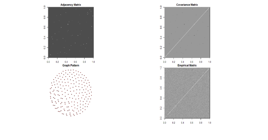
Simulated datasets with different dimensions p of multivariate normal distributed response Y, number of observations n, and five predictors were generated. The case presented in Figure 1 a-d is data with dimension p=200, n=100, and no of edge = 31. The other cases with different p, n and number of edges were presented in the supplementary information.

Figures 1a-1c presented the graphical profiling of the relationships between different MLS variance estimates 𝜽̂ of β based on GGM graph structure across different penalty parameter λ in one of the simulation cases. These variance estimates used either a penalized precision matrix or a penalized variance-covariance matrix of the multivariate response variable Y, in a range of the penalty tuning parameter λ. All the graphs present the ratio (𝜽̂ /𝛉) of a derived β’s variance 𝜽̂ to the known population variance θ.

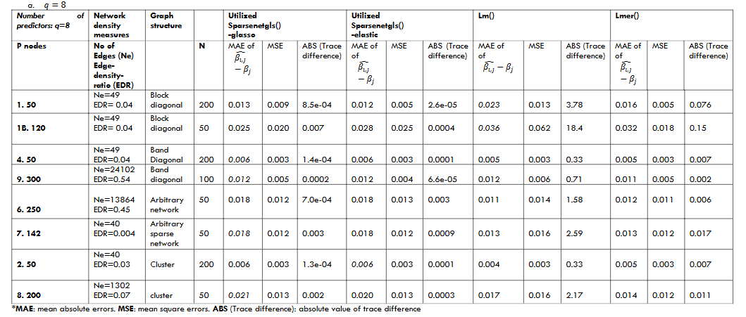
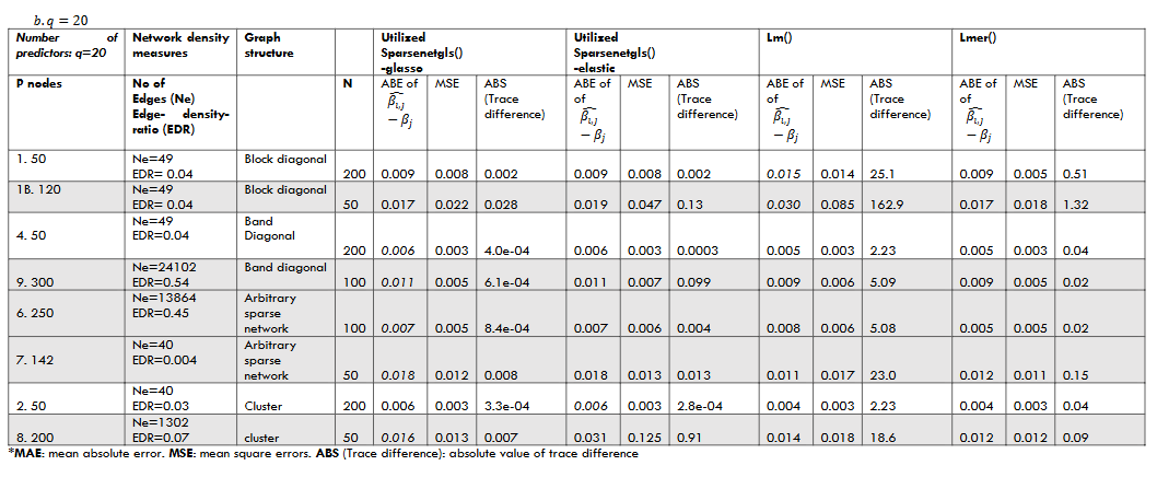
3.2 SIMULATIONS TO COMPARE FUNCTIONS: sparsenetgls(), lm() (linear regression) and lmer() (mixed effect linear regression)

3.2.1 Design and measures for model comparison

Multivariate response data 𝐘 with different p (number of dimensions), n (number of subjects), and explanatory variables X with different q (number of dimensions) were simulated given a known regression coefficient vector 𝜷. Simulations were conducted using R huge package to provide different graph structures (block, cluster, band diagonal, random) of the precision matrix for the response variable Y. The simulated response and explanatory variables were included in the sparenetgls GGM- MLS. The sparsenetgls 𝛃̂ was a weighted estimate of a precision matrix (Ω̂) derived from different penalized GGM methods. The estimation of β’s variance-covariance matrix 𝛤̂, was using the penalized Ω̂ with the minimal informatic criteria and the penalized covariance matrix Σ̂ (λ) with the graph complexity, selected through the second tuning parameter d. The penalized covariate matrix of the multivariate responses Y was initially converted from the mid-point solution of the network graph structure series represented by the precision matrix series. Σ̂ was further derived through the second tuning parameter d. The variance-covariance matrix 𝛤 used in the trace comparison was derived based on the known 𝐘 ‘s variance-covariance matrix Σ and the limiting distribution of the penalized precision matrix Ω_λ.

The measures we used to compare the different estimates to the known values were the average absolute deviation (mean absolute error: MAE) in 1/𝑞 ∑_𝑞𝑗∑ |(𝛽̂_𝑖,𝑗−𝛽_𝑗)|_{𝑖𝑡𝑒𝑟𝑛𝑜}𝑖_{𝑖𝑡𝑒𝑟𝑛𝑜}. Mean square error (MSE), and the absolute trace difference where q was the number of explanatory variables, j represented the jth explanatory variable, and i was the ith iteration. The average deviation from 𝛽 was calculated by averaging the deviation of each element 𝛽_𝑗 in the repetitions and then averaged across q elements. The trace difference was derived between 𝛤 and the 𝛤̂ (i.e., 𝛽̂ ‘s sample variance-covariance matrix) from sparsenetgls.

In the simulations, the edge-to-density ratio, defined as the ratio between the number of edges to graph density, was used to measure the sparsity of the network graph. There is no universally defined sparsity for a network. The general agreement is that if the number of edges is on the same linear scale as the number of all possible links (p*p/2), it is a dense network. The cases in the simulation studies have included both sparse (with edge-to-density ratio of less than 0.10) and dense networks. All the results presented in Table 1 were generated from 100 repetitions.

3.2.2 Impact of the number of observations

Different simulation cases suggested that when n increased, the deviation between the estimated 𝛽̂ and actual value 𝜷 decreased in all estimation methods. The differences between the trace of 𝛤̂ and the limiting distribution (actual) 𝛤 were also smaller when n increased in all methods.

3.2.3 Comparing regression coefficient estimates of GGM-MLS (via sparsenetgls) and their variance to lm and lmer

The deviations between the sample estimate 𝛽̂ and actual 𝛽 varied across different patterns of the graph structure. The MAE in the regression coefficients between sparsenetgls, lm and lmer have both directions (smaller or larger) with trivial differences, with similar estimates between sparsenet and lmer. However, the MSE and abs (Trace difference) were smaller in sparsenetgls than lm and lmer in all simulations. In summary, compared to the actual value 𝛽, the deviations in the GGM-MLS regression coefficient estimates were trivial in all the simulated cases; they were all less than 3.0 % of the actual values. Using GGM in the estimation of MLS regression coefficients 𝛽 could improve the estimation in networks with smaller variance (i.e., improve the precision). The simulation results were consistent with the asymptotical orthogonality feature of Ω and β (presented in supplementary information), i.e., the estimation of the precision matrix Ω does not affect the estimation of the MLS regression coefficients when n is sufficiently large; they are two independent processes. The variance and standard errors derived from the GGM-MLS were smaller than those derived from lm and lmer.

3.2.4 Prediction accuracy in the graph structure:

Before utilizing the GGM approach in MLS, simulations were also used to compare the prediction accuracy in graph structure using glasso, and elastic-net methods. Figure four (in supplementary information) demonstrated four different scenarios when p and n differed. All three cases showed that glasso had a higher AUC (better accuracy) than the other approximation approaches. However, the lasso and elastic methods were better when n was much larger than p in the second case.

4. Case studies:

4.1 CASE STUDY ONE AND TWO

The two case studies used Copy Number Alteration information from 77 breast cancer patients to predict the related proteins’ abundance. The proteins were chosen according to an immune response association network from the publication of the same study. The first network has 29 proteins corresponding to immune response, and the Copy Number Alterations (CNA) information was chosen from 8 genes reported to be clinically relevant and related to breast cancer. The second network has 69 proteins of the calcium ion binding network.

The analytical methods: Firstly, the developed “sparsenetgls” function was used to derive the GGM-MLS regression coefficient 𝛃. The precision matrix of the graph structure was estimated using the glasso method, the covariance matrix was determined by the penalty parameter λ and the tuning parameter d. The selection of 𝛃 was based on the information criteria (i.e., solution I) and the minimal variance (i.e., solution II). Secondly, multilevel model through Linear mixed effect models (lmer), with only variance information included, were used to derive the fixed effect coefficients. These results were compared in terms of regression coefficients and their standard errors.

In case study one, the regression coefficients of the significant genes GATA6, TP53BP1, TP53L11 from solution II in GGM-MGLS were not much different from the results of lmer. Nevertheless, the regression coefficients from solution I showed larger differences than the results of lmer. Based on the 95% confidence intervals of the regression coefficients, Gene TP53BP1 was significantly associated with the protein abundance of the immune response network in both GGM-MLS solutions but only indicated marginal significant in the lmer results.

In the second case study, we used the same dataset but a more extensive network of 64 calcium ion binding proteins; the protein abundance predictors are copy number alteration (CNA). Similarly, the regression coefficients of the significant genes GATA6, PGR, PIK3CA, TP53BP1, TP53IL1, and TP53INP1 from solution II were also not much different from lmer when the precision matrix was selected using the minimal informatic criteria, but presented larger difference from the solution I.

The other findings were that CNA of gene PIK3CA and TP53INP1 were significantly associated with the abundance of proteins in the calcium ion network in the GGM-MLS results solution I. However, the association was not significant in solution II and was marginally significant in lmer.

In both cases, the standard errors of the regression estimate in solution I (minimal beta variance) were smaller than in solution II (minimal-informatic criteria) and lmer. When the number of observations is sufficiently large, we expect the regression coefficients from these functions to converge to the population estimates. The standard error derived from GGM-MLS with the minimal variance option is more sensitive; as such, the results could be more prone to type I errors. However, GGM-MLS and lmer solutions help derive comparative regression coefficients, with smaller standard errors from GGM-MLS.

4.2 The case study three: a large protein network of CBNT case

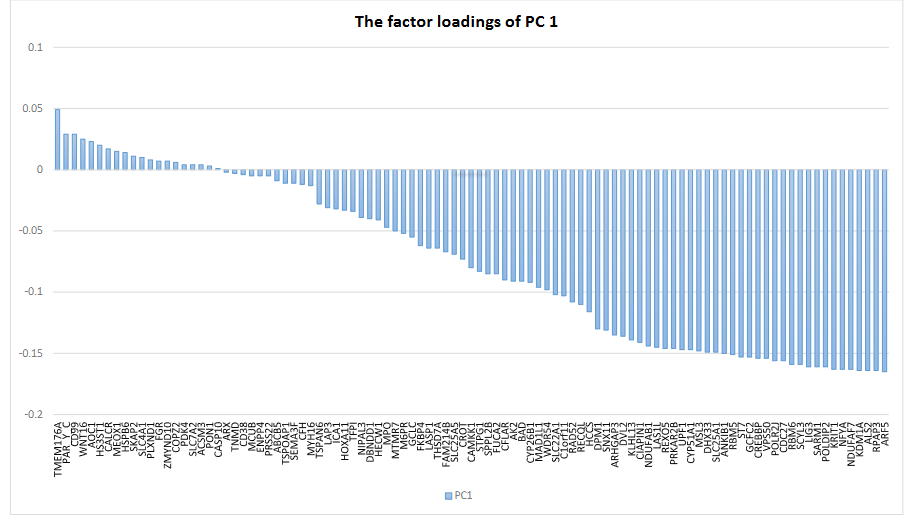
Fifty patients diagnosed with brain tumour Ependymomo’s Gene expression data of Kallisto quantified transcript abundance and RSEM quantified gene expression were selected from 282 patients’ sample (PedcBioPortal KidsFirst (kidsfirstdrc.org)). Gene expression of 100 candidates was included as predictors of 200 selected gene’s transcript abundance, principal component analysis was conducted and reduced the data dimensions to 20 significant principal components (PCs); the first PC explained 30% variance of the gene expressions. Using sparsenetgls, the first PC of gene expression presented significant associations with the multivariate distributed abundance data. Twenty genes had high negative loadings within the first principal component on the first PC, indicating their potential impacts on protein quantifications.

5. Discussion

Gaussian Graphical Model multivariate linear regression, including the graphical estimations of the precision and variance-covariance matrix of multivariate response data, improves the estimations in multivariate regression. In the scenario of n<p, GGM-MLS is more advantageous because sparse induction in the covariance matrix becomes necessary.

The first case study using the suggested model found significant association between Copy number alternation of gene TP53BP1 (Tumor Protein P53 Binding Protein 1) and the abundance of immune response proteins. TP53BP1 gene encodes a protein that has multiple roles in DNA damage response. The second case study discovered significant associations between copy number alternation of genes GATA6, PGR, PIK3CA, TP53BP1, TP53IL1, TP53INP1 and the abundance of proteins in calcium ion binding network. Gene GATA6 is in the small family of zinc finger transcription factors that play an important role in the regulation of cellular differentiation and organogenesis during vertebrate development. Gene PGR encoded protein that mediates the physiological effects of progesterone, which plays a central role in reproductive events associated with the establishment and maintenance of pregnancy. Gene PIK3 is an important oncogene that most recurrently mutated in breast cancer and its mutation will contribute to cancer cell growth. The other TP genes are related to tumour cells; and gene TP53INP1 is a tumor cell depressor which was found to downregulate the abundance of proteins in calcium ion network.

Simulation studies and analytical evidence suggest that the influence of penalized precision matrix of the response variables on regression coefficient estimates of multivariate gls (MLS) is trivial when n (the number of observations) is sufficiently large and greater than p (the number of dimensions of the response variable). The influence of the graph structure (i.e., non-zero covariance term) is nontrivial on the variance estimates of the regression coefficients. When n < p, the penalization of the precision matrix is efficient and necessary to derive the MLS regression coefficients and their variance.

Based on the uniqueness of the precision matrix property described in Dempster (1972), the network graph structures estimated from the precision matrix and the variance-covariance matrix should be the same. However, according to empirical evidence, penalization of the precision matrix was shown to be more effective than using penalization of the variance-covariance matrix in deriving the variance-covariance matrix 𝛤̂ of the MLS regression coefficients.

Limitations of the study included the computation capacity restricted the number of observations in the simulations to less than 1000 but reflective of most studies in omics and high throughput studies. The simulations only presented results of the “glasso” and “enet” options in “sparsenetgls”. More studies are required to test other GGM approaches in the future.

Future studies that use GGM for deriving regression coefficients of mixed model regression with different covariance structures in correlated predictors and with large categorical network-linked outcome data will be promising.

6. Conclusion

Integrating Gaussian graphical model estimator in high-dimensional outcome analysis using multivariate linear regression provide an unbiased solution with better precision. Implications of the GGM-MLS method in medical research include an expansion of evaluating outcome measurements in the large dimensional space, and allowing latent patterns of the high-throughput outcomes included in treatment evaluations, diagnosis testing and prediction. These latent patterns, which potentially present the biological, physiological and psychological functionality and connections, could enrich information of the outcome measures in the analysis.

Data Availability Statement

Acknowledgement Data used in this publication were generated by the Clinical Proteomic Tumor Analysis Consortium (NCI/NIH). They were obtained as part of the CPTAC DREAM Challenge project-2017 through Synapse. This research was supported by the National Cancer Institute (NCI) CPTAC contract 16XS230 through Leidos Biomedical Research, In. Similar datasets can be applied from: https://proteomics.cancer.gov/data-portal. The research (case study 2) was conducted using data made available by The Children’s Brain Tumor Network (CBTN). The authors also wish to acknowledge the facilities and supports provided by the eResearch Infrastructure NZ (www.nesi.org.nz).

References

1. Yamashita A, Sakai Y, Yamada T, et al. Generalizable brain network markers of major depressive disorder across multiple imaging sites. Plos Biology. 2020;18(12)
2. Cai M, Chen J, Hua C, Wen G, Fu R. EEG emotion recognition using EEG-SWTNS neural network through EEG spectral image. Information Sciences. 2024/10/01/ 2024;680:121198. doi:https://doi.org/10.1016/j.ins.2024.121198
3. Royer J, Rodríguez-Cruces R, Tavakol S, et al. An Open MRI Dataset For Multiscale Neuroscience. Scientific Data. 2022/09/15 2022;9(1):569. doi:10.1038/s41597-022-01682-y
4. Borsboom D, Deserno MK, Rhemtulla M, et al. Network analysis of multivariate data in psychological science. Nature Reviews Methods Primers. 2021/08/19 2021;1(1):58. doi:10.1038/s43586-021-00055-w
5. Van der Vaart AW. M- and Z-Estimators. Asymptotic Statistics. Cambridge University Press; 1998.
6. Goldstein H. Multilevel statistics model John Wiley & Sons; 2010.
7. Zeng IS, Lumley T, Ruggierol K, Middleditch M. A Bayesian approach to multivariate and multilevel modelling with non-random missingness for hierarchical clinical proteomics data. 2017.
8. Zeng IS. Topics in Study Design and Analysis for Multistage Clinical Proteomics Studies. In: Jung K, ed. Statistical Analysis in Proteomics. Springer; 2016.
9. Pinheiro JC, Bates DM. Mixed-effectS models in S and S-PLUS Statistics and Computing. Springer; 2007.
10. Miller RG. The Jacknife – a review. Biometrika. 1974;61:1-15.
11. Yuan M, Lin Y. Model Selection and Estimation in the Gaussian Graphical Model. Biometrika. Mar 2007;94(1.):19-35.
12. Friedman J, Hastie T, Simon N, Tibshiran N. Regularization Paths for Generalized Linear Models via Coordinate Descent. Journal oF Statistical Software. 2010;33(1)
13. Friedman J, Hastie T, Tibshirani R. Applications of the lasso and grouped lasso to the estimation of sparse graphical models. 2010.
14. Meinshausen N, Buhlmann P. High-dimensional graphs and variable selection with the lasso. The annals of statistics. 2006;34(3):1436-1462.
15. Peng J, Wang P, Zhou N, Zhu J. Partial Correlation Estimation by Joint Sparse Regression Models. Journal of the American Statistical Association. 2009;104(486):735-746.
16. Cai T, Li H, Liu W, Xie J. Covariate-adjusted precision matrix estimation with an application in genetical genomics Biometrika. 2013;100:139-156.
17. Zhang J, Li Y. High Dimensional Gaussian Graphical Regression Models with Covariates. Journal of the American Statistical Association. 2022;0(0)
18. Devijver E, Gallopin M. Block-Diagonal Covariance Selection for High-Dimensional Gaussian Graphical Models. Journal of the American Statistical Association. 2018;113(521):306-314.
19. Bondy JA, Murty USR. Directed graphs. Graph theory with applications. Elsevier Science Publishing Co. Inc 1976.
20. Zhao T, Liu H. The huge Package for High-dimensional Undirected Graph estimation in R. Journal of Machine Learning Research. 2012;13: 1059-1062.
21. Hurley N, Rickard S. Comparing measures of sparsity. IEEE Transactions on Information Theory,. 2009;55(10):4723-4741.
22. Mertins P, Mani DR, Ruggles KV, et al. Proteogenomics connects somatic mutations to signalling in breast cancer. Nature. 2016;534:55-73.
23. National Library of Medicine.
24. Seillier M, Peuget S, Gayet O, et al. TP53INP1, a tumor suppressor, interacts with LC3 and ATG8-family proteins through the LC3-interacting region (LIR) and promotes autophagy-dependent cell death. Cell Death & Differentiation. 2012/09/01 2012;19(9):1525-1535. doi:10.1038/cdd.2012.30