The Impact of Covid-19 on Higher-Age Mortality

Andrew J.G. Cairnsa ^1*, David Blakeb ^2, Amy R. Kesslerc ³, Marsha Kesslerd ⁴

1. Maxwell Institute for the Mathematical Sciences and Heriot-Watt University, Edinburgh
2. Bayes Business School, City St George’s, University of London
3. Prudential Financial
4. M Kessler Group

OPEN ACCESS

PUBLISHED: 31 January 2025

CITATION: Cairns, A. J. G, Blake, D., et al., 2025. The Impact of Covid-19 on Higher-Age Mortality. Medical Research Archives, [online] 13(1). https://doi.org/10.18103/mra.v13i1.6186

COPYRIGHT: © 2025 European Society of Medicine. This is an open-access article distributed under the terms of the Creative Commons Attribution License, which permits unrestricted use, distribution, and reproduction in any medium, provided the original author and source are credited.

DOI: https://doi.org/10.18103/mra.v13i1.6186

ISSN 2375-1924

ABSTRACT

We propose a simple model for accelerated deaths that draws on the observation that many of those who died from Covid-19 were often, but not always, much less healthy than the average for their age group; further, the vast majority who died were over the age of 50. The model predicts that, in the absence of additional secondary effects, the impact on the life expectancy of survivors (the anti-selection effect) will be very small, and that the degree of impact depends on the average years of life lost by those who die from Covid-19. The philosophy underpinning the model is supported by reference to both all-cause mortality by age and all-cause mortality by socio-economic deprivation group. In combination, these support a proportionality link between Covid-19 mortality and individual frailty or death rates. The Accelerated Deaths Model is consistent with the mortality experience associated with respiratory diseases over the period 2013-15 and with past seasonal influenza epidemics.

Keywords: Covid-19, all-cause mortality, frailty, co-morbidities, deprivation, Accelerated Deaths Model, Proportionality Hypothesis, anti-selection.

1. Introduction

Covid-19, the novel coronavirus that began in Wuhan in China in late 2019 and circumnavigated the Earth in a matter of weeks, creating the worst global pandemic since Spanish Flu in 1918-19, has had the greatest impact on those aged over 50, particularly males as Figure 1 shows in the case of England & Wales.

Covid-19 kills by inflaming and clogging the air sacs in the lungs, depriving the body of oxygen ‒ inducing hypoxia ‒ other essential organs. The virus can also lead to heart inflammation (e.g., myocarditis), irregular heart rhythms risking cardiac arrest, kidney, liver and intestinal damage, blood clots (which can lead to stroke or pulmonary embolism), and neurological malfunction. This can be exacerbated by the immune system which fails to stop when the threat has passed. Around half of patients hospitalized with Covid-19 have blood or protein in their urine, indicating damage to their kidneys. Up to 30% of intensive-care patients lose kidney function and require a form of dialysis called continuous renal replacement therapy. Many Covid-19 patients with existing illnesses related to lungs, kidneys, etc who went into intensive care failed to survive. However, some surviving intensive care patients developed a new life-shortening impairment (e.g., related to organ damage) that they did not have before.

The aim of this paper is to develop a model and scenarios for the potential direct impact of Covid-19 on higher-age mortality, once the pandemic has run its course. We seek answers to the following questions. How many of the deaths directly caused by Covid-19 would have happened in the relatively near future in any event because those infected by the virus were frail and had serious existing illnesses (or co-morbidities) which meant that they had a shorter life expectancy relative to their peers even if they had not caught the virus? In other words, what is the impact on the average life expectancy of the general population after the pandemic? We will argue that the answers to these questions will depend on the following key variables: age, gender, and socio-economic status of infected individuals, as well as the infection rate in their vicinity.

There are also questions related to the indirect impact of Covid-19:

• How many people who recovered from Covid-19 developed an impairment, such as organ damage, that they did not have before and which shortened their life expectancy? This is likely to be related to the number of infected people who needed intensive care in hospital.
• How many people who self-isolated during the pandemic did not then seek timely medical diagnosis or treatment for other conditions during the pandemic, e.g., cancer, and developed more serious cases as a result, which could reduce their life expectancy?
• How many people will have their life expectancy reduced ‒ because of an increase in alcohol/drug consumption and suicide, as a consequence of self-isolation or long-term unemployment if the economy remains in recession for an extended period and/or many more jobs are automated in response to the pandemic?
• How many people will permanently change their social behaviour or seek treatments that delay the impact or onset of age-related diseases, one of the primary factors that make people more susceptible to the virus both of which could have the effect of increasing their life expectancy?

We will specify some simple scenarios to capture some of these issues in a broad brush sense. In due course, if and when the relevant information becomes available, then the Accelerated Deaths Model (ADM) could be extended and/or modified to address these questions more fully.

The outline of the paper is as follows. Section 2 discusses methodology, data and possible scenarios. In Section 3, we calibrate a simple two-parameter ADM using plausible assumptions. In Section 4, we specify some plausible Covid-19 scenarios. In Section 5, we calibrate the model to account for age dependency in one of its parameters. In Section 6, we calibrate the model to account for socio-economic differences in mortality. Section 7 considers the observable consequences of accelerated deaths with lessons from the pattern of deaths from previous respiratory diseases: in particular, the model predicts higher death rates during the pandemic, followed by lower death rates after the pandemic due to anti-selection before gradually reverting to previously predicted levels of mortality. Section 8 looks for lessons from past seasonal influenza epidemics, while Section 9 considers the indirect impacts of the Covid-19 pandemic. We end with a discussion in Section 10 and a conclusion in Section 11.

2. Methodology, Data and Scenarios

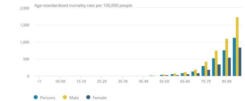
To address these questions, we need to make assumptions about models, data and scenarios. We choose to use a standard model of mortality, the Gompertz model (Gompertz (1825)), and develop plausible scenarios using a simple model for accelerated deaths. The left-hand panel of Figure 2 shows, for a particular age cohort, the impact on the cohort aggregate deaths curve if Covid-19 deaths are randomly distributed across the age range, while the right-hand panel shows the impact if the Covid-19 deaths are front-loaded and affect more those who are currently less healthy (and have more co-morbidities) than the average for this age cohort. Since around 97% of deaths occur above the age of 50, we concentrate on this age range which also happens to be the age range over which the Gompertz model fits well. In terms of country, we use data from EW and comment briefly on an application of the model to US data although the model is general enough to be adapted for use in all countries.

We are interested in the total impact of the pandemic, so we assume that all Covid deaths occur at the start of the pandemic. In order to calibrate the ADM, we need answers to the following questions:

• What will be the total number of deaths over the course of the pandemic?
• What will be the age distribution of the deaths?
• What will the gender split be?
• What will be the split between socio-economic sub-groups?
• How much of the differences between these sub-groups can be explained by differences in all-cause mortality?

To answer the first question, we could wait until the pandemic had run its course. We could then calibrate the ADM to match exactly the total number of Covid deaths as well as the actual shape of the grey area in the right-hand panel of Figure 2: we denote this the ex-post ADM. Alternatively, we could estimate the number of deaths based on expert judgement at the start of the pandemic and combine this with plausible scenarios about the likely impact of the pandemic: we denote this the ex-ante ADM.

We decided to build the ADM as though we were near the start of the pandemic (May 2020), i.e., the ex-ante version. At that time, a reasonable estimate was that there would be around 75,000 to 85,000 deaths in EW if social distancing measures were maintained. There was also reasonable data on the gender split and the age distribution and there was some information on socio-economic differences. The ex-ante ADM therefore concentrated on the relationship between existing co-morbidities (frailties) and Covid-19 deaths.

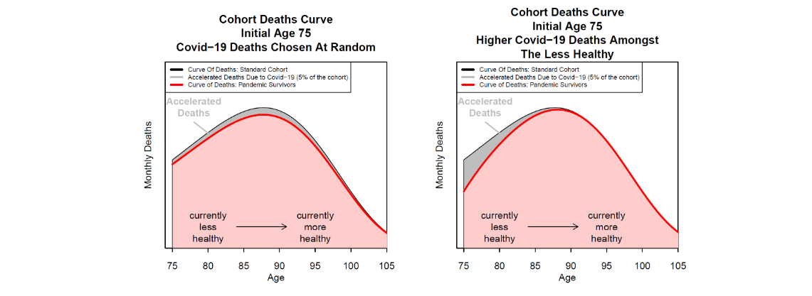
A particularly important finding for calibrating the ADM highlighted by Professor David Spiegelhalter and other commentators was the approximately parallel relationship between the log of non-Covid-19 death rates and age and the log of Covid-19 death rates and age (in both cases above age 30), implying that Covid-19 mortality seems to be proportional to all-cause mortality at adult ages (see Figure 3). In other words, Covid-19 mortality rate is proportional to all-cause mortality rate in a normal non-Covid year.

3. The Accelerated Deaths Model of the Direct Impact of Covid-19 on Higher-Age Mortality

We use the near-parallel relationship in Figure 3 to investigate the link between Covid-19 and frailty by age as measured by all-cause death rates: Covid-19 mortality rate(𝑥) = All-cause mortality rate(𝑥) × Infection rate(𝑥) × Relative frailty(𝑥). The evidence indicates that a significant proportion of people who die from Covid-19 are in a frail state. Figure 4 for EW, for example, shows that those who died had significant co-morbidities, in particular, ischaemic heart diseases, dementia and Alzheimer’s disease, influenza (flu) and pneumonia, and diabetes. Only a small percentage (Figure 4: 7-12% depending on subgroup) had no pre-existing conditions. Data for New York State are consistent with this: only 11% of those who died had no co-morbidities.

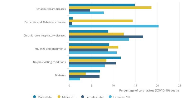
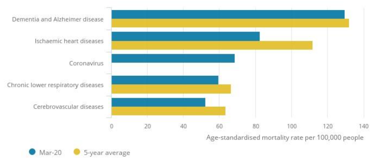
Figure 5 shows that the four main causes of death during March 2020, apart from Covid-19, were ischaemic heart diseases, chronic lower respiratory diseases, and cerebrovascular disease. A possible inference of Figures 4 and 5 is that Covid-19 deaths can be broken down into three groups:

• deaths of people who have one or more co-morbidities and would have died from these in the relatively near future, had they not contracted Covid-19;
• deaths of people who have one or more co-morbidities, but would have been expected to live beyond 2020 had they not contracted Covid-19 (perhaps for many years); and
• deaths of people (between 7-12% according to Figure 4) who had no co-morbidities and who would otherwise have had a longer life expectancy, perhaps consistent with the average for their cohort.

The data in Figures 4 and 5, therefore, lend weight to the view that some of those who died from Covid-19 would have died in the near future anyway. Sadly, a number would have lived for rather longer, with between 7-12% potentially living significantly longer had they not contracted the virus.

Further evidence comes from Docherty et al (2020) who report that, on the basis of the ISARIC WHO Clinical Characterisation Protocol, 53% out of their sample of 16,749 UK people hospitalized due to Covid-19 had significant co-morbidities. This is an overlapping but not identical pool of patients, but the difference between co-morbidities at admission and death indicates a strong link between prior health and ability to survive hospitalization. We therefore propose the following Accelerated Deaths Hypothesis: Some of those who die from coronavirus would have died anyway in the relatively near future due to these co-morbidities. Within a given cohort, Covid-19 deaths will, therefore, be more prevalent amongst people who already had a shorter expected lifetime (due to these co-morbidities) compared to the average for the cohort.

The model that we propose below is speculative and highly stylized. Its purpose is to explore the possible impacts of the pandemic. If and when additional mortality experience data become available, the model can be refined, including detailed calibration to different populations. We also reiterate the point that we are not attempting to model the path of the epidemic itself, just the aftermath. The simple model is also limited to ages 50 and above.

3.1 MODEL A: BASELINE MORTALITY MODEL

We calibrate our baseline model for mortality (in the absence of the pandemic) to EW. We assume that the period life table for death rates follows a Gompertz function with a growth rate 0.105 and a death rate of 0.01 at age 65. The assumed long-term mortality improvement rate is 1.5% per annum at all ages. Projected deaths are calculated on a monthly basis. We will therefore write dA(t, x) = aggregate deaths in month t for a cohort with initial size 100,000 and initial age x. As a function of t, dA(t, x) defines what we refer to as the baseline cohort aggregate deaths curve.

3.2 MODEL B: ACCELERATED DEATHS MODEL DUE TO COVID-19

The ADM is an adjustment to Model A to account for those lives within the cohort that are likely to die of Covid-19. For each age cohort, deaths are divided into two groups: those who die from Covid-19 and those who either survive the infection or are not infected at all. Specifically, we assume that out of the dA(t, x) deaths expected or scheduled to die in month t, a proportion, π(t, x), will die from Covid-19. The shape of π(t, x), as a function of t, is chosen to reflect the observation that most people who die from Covid-19 have existing significant co-morbidities. The shape of π(t, x) needs to reflect the shape of the grey area in the right-hand panel in Figure 2 and a simple functional form for achieving this is a two-parameter decreasing exponential function of π(t, x).

π(t, x) = α(x) / ρ(x) exp[-t/(12ρ(x))]. Although this functional form is purely judgemental, it captures the idea that people who are expected to die sooner rather than later are more likely also to die from Covid-19 if they have contracted the virus. Other forms for π(t, x) could equally be plausible, but the exponential form is simple and easy to understand.

The parameter α(x) defines what we call the amplitude (or impact) of the effect at age x. As an approximation, α(x) measures the number of Covid-19 deaths as a proportion of expected deaths due to all causes at age x (i.e., in the next year). The parameter ρ(x) is what we call the reach of the accelerated deaths. As an approximation, the reach measures the expected remaining years of life lost (i.e., remaining life expectancy) by those who die immediately from Covid-19. As a group, they would have otherwise lived, say, 85, then YLL will be greater than the reach. If the reach is increased to infinity then anti-selection disappears completely and the ratios plotted in Figure 9 would drop back to exactly 1 at all ages and the left-hand figure of Figure 2 would apply.

Covid-19 deaths in month 1 for the cohort currently aged x (per 100,000) are thus dC(x) = ∑ π(t, x)dA(t, x) t, and the curve of deaths for survivors of the pandemic is dS(t, x) = (1 – π(t, x))dA(t, x) for t = 1, 2, … .

To demonstrate how the model works and the effects on life expectancies, we begin with an extreme-mortality scenario in which we assume 500,000 deaths when we adjust cohort sizes to match the approximate 20 million people in the age range 50-100 in EW. This corresponds to the worst-case scenario predicted by the Imperial College Covid-19 Response Team assuming no government intervention to slow down the spread of the pandemic.

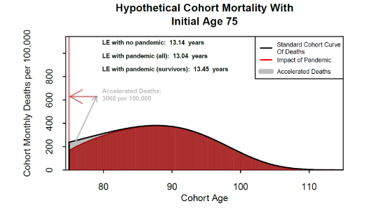
Figure 6 illustrates the ADM in this worst-case extreme-mortality scenario. The black curve represents expected monthly deaths (for an initial cohort size of 100,000, all aged 75) in the absence of Covid-19. The grey triangular area represents the people who die from Covid-19 (3,060 per 100,000 in this example). The shape of π(t, x), multiplied by dA(t, x) dictates the shape of the grey region. The vertical red bar on the left counts all Covid-19 deaths over the pandemic (the bar begins at 180 which is the assumed regular death count in month 1). The red area illustrates the cohort (either because they were not infected or they recovered). The modified red area and the associated mortality curve results in a form of anti-selection. The shape of the red curve implies that survivors are, on average, healthier than the average for the cohort before the pandemic and so have lower average mortality, but their future mortality experience gradually reverts over time (depending on the size of ρ(x)) to standard mortality.

Some survivors, most likely those who needed intensive care, could end up with a new impairment, such as organ damage, which will reduce their life expectancy. However, for survivors as a whole, we conjecture that their life expectancy has increased relative to their age cohort before the outbreak of the pandemic. In our example, the life expectancy of 75-year old survivors increases from 13.14 to 13.45, while the life expectancy for the whole cohort (because of premature Covid-19 deaths) falls to 13.04 from 13.14. It is important to note that these differences ‒ which measure the magnitude of the anti-selection effect ‒ are very small.

The effect on accelerated deaths of a change in the amplitude, α(x), is straightforward. For example, doubling α(x) doubles the depth of the grey region in Figure 6 and doubles the number of accelerated deaths.

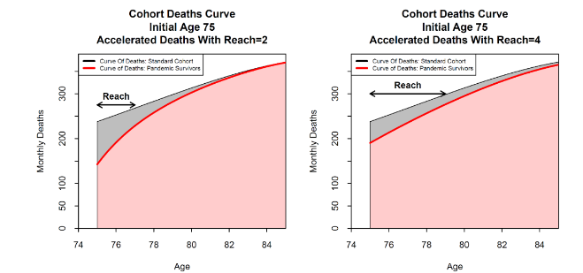
Figure 7 shows the effect of a change in the reach, while keeping the amplitude fixed. The left and right-hand plots show the impact of extending the reach from 2 to 4 years. The grey area with the accelerated deaths narrows at the left-hand end, but stretches out to the right. The total number of deaths remains approximately the same (since the amplitude is fixed), but the expected years of life lost by the Covid-19 victims approximately doubles. Additionally, increasing the reach reduces the magnitude of the anti-selection in a given year.

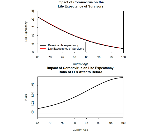
In Figure 8, for the same extreme-mortality scenario as Figure 6, we look at the effect on life expectancies. In the top plot, the small difference between the black and red lines is only just visible. The bottom plot shows the same relationship expressed as a ratio which makes the consequence of the pandemic clearer: the anti-selection effect means that survivors have an increase in life expectancy of between 1% at age 65 rising to over 6% at age 90.

4. Specifying Plausible Covid-19 Scenarios

In light of the UK’s lockdown policy and assuming social distancing measures are maintained after the lockdowns are lifted, we take as our best estimate 75,000-85,000 Covid-19 deaths for EW, which is less than 20% of the worst-case scenario, but close to the 73,766 who actually died from Covid-19 in EW in 2020, during the first year of the pandemic. In the scenarios that follow, we will calibrate the amplitude and reach parameters so that the model generates approximately 80,000 accelerated deaths. The ex-post ADM will, of course, be based on the final number of Covid-19 deaths, although it might never be known how many deaths due to Covid-19 were incorrectly reported.

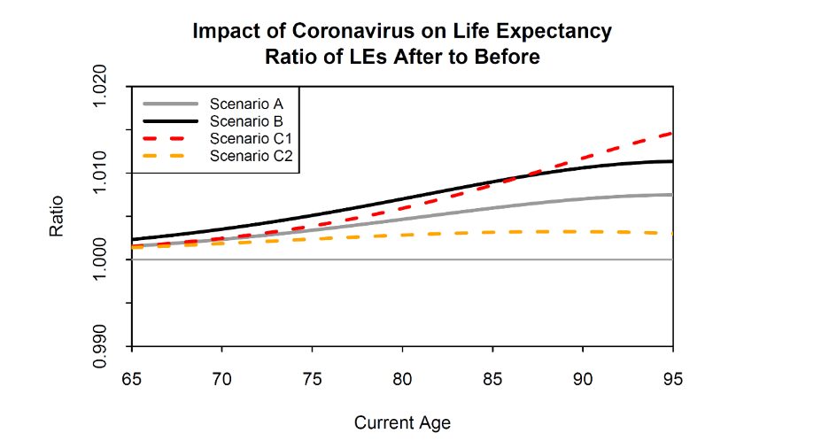
In our new baseline case (Scenario A see Table 1), we will assume that α(x) = 0.14544 and ρ(x) = 4 for all x. This implies that, at all ages, approximately 14.5% of all deaths over the next year are assumed to be due to Covid-19, while those who die of Covid-19 lose approximately 4 years of life. We consider three additional scenarios:

• Scenario B sets α(x) = 0.21816 and ρ(x) = 4, for all x.
• Scenario C1 sets α(x) = 0.14228 and ρ(x) = 2, for all x.
• Scenario C2 sets α(x) = 0.15152 and ρ(x) = 8, for all x.

The effect on life expectancies under the four scenarios A, B and C1 and C2 is illustrated in Figure 9. For the baseline Scenario A, we can see that, unsurprisingly, the effect of anti-selection on life expectancies is much smaller than in Figure 8. At younger ages, life expectancies rise by only about 0.2%, compared with 1% in Figure 8. When we double the amplitude (Scenario B), the effect on life expectancies doubles at all ages. When we halve the reach (Scenario C1), the shape of the curve in Figure 9 changes, but the effect on life expectancies remains similar. When we double the reach (Scenario C2), the curve moves closer to that of scenario A. A key conclusion is that, with 80,000 Covid-19 deaths in England & Wales, the impact on the life expectancy of survivors is likely to be very modest.

Table 1: Scenarios considered

Scenario	Accelerated deaths function, π(t, x) (Equation (2))	Age-related amplitude function, α(x) (Equation (3))
A	0.14544	4
B	0.21816	4
C1	0.14228	2
C2	0.15152	8

5. Calibrating the Model to Account for Age Dependency in the ADM’s Parameters

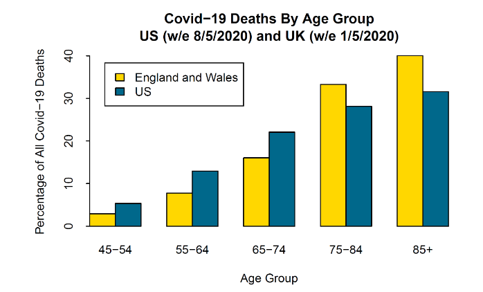
To motivate this, we compare registered deaths in EW and the US. Figure 10 shows the age profile of Covid-19-registered deaths in EW versus the US. It can be seen that the shapes of the EW and US profiles are quite different with, in relative terms, a much higher proportion in the US of deaths in the 50s and 60s ‒ a difference that cannot be explained by differences in the age profiles of the two populations. This might be due to differences in the degree of social distancing at different ages in the two countries. Another possible reason relates to differences in the healthcare systems. In the US, infection rates might be the same as the UK, but poor access to high-quality healthcare for the more deprived in the US population might push up Covid-19 death rates. After age 65, access to Medicare in the US might mitigate this, but health challenges persist for those who were underinsured or uninsured during their working lifetimes and a gap persists in the quality of healthcare between those reliant on Medicare versus those with supplementary private healthcare in retirement.

For our model to produce a reasonable match to both EW and the US, we need to allow the amplitude to vary with age. We, therefore, introduce two new scenarios, D and E, where, instead of being constant, α(x) follows a logistic function of age x:

α(x) = α1 + (α0 − α1) / (1 + exp((x−x0)/λ)). The function starts with an amplitude equal to α0 at low ages, transitioning smoothly up (if α0 > α1) or down (if α0 < α1) to a new level of α1 at high ages. The two new scenarios are (see Table 1):

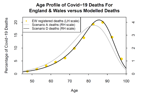
• Scenario D sets x0 = 83, λ = 5, α0 = 0.1032 and α1 = 0.2064, with ρ(x) = 4 for all x: a low amplitude at low ages gradually shifts to a higher amplitude at high ages, relative to Scenario A.
• Scenario E sets x0 = 70, λ = 5, α0 = 0.2304 and α1 = 0.1152, with ρ(x) = 4 for all x: a high amplitude at low ages gradually shifts to a lower amplitude at high ages, relative to Scenario A.

Compared with Scenario A, Scenario D results in fewer deaths at the younger ages and more deaths at the high ages: see Figure 11, grey and black lines. Figure 11 also shows the age profile for registered deaths in EW. We can see a significant difference between Scenarios A and D, with Scenario D (black line) providing a much better match to the EW data (gold dots). Scenario E (not plotted) shifts the balance in the other direction from Scenario A towards younger ages rather than old. Scenario E happens to fit US data well up to the 75-84 age group, but underestimates deaths in the 85+ age group, indicating that the form of α(x) in Equation (3) needs to be modified to fit the data of other countries better.

6. Calibrating the Model to Account for Socio-Economic Differences in Mortality

We now explore a different facet of the data that has been published by the UK Office for National Statistics (ONS) concerning the distribution of deaths across different socio-economic groups. Media reports in the UK at the start of the pandemic suggested that members of lower socio-economic groups were more likely to contract Covid-19 than those in higher groups. This is because the former live in more crowded dwellings in poorer neighbourhoods and were more likely to have to leave home and travel on crowded public transport in order to go to work (especially in the health and care sectors), while the latter were more likely to be able to work from home and exercise in private gardens or spacious parks, thereby reducing the risks of catching the virus. If the infections resulted in relatively more deaths, this could widen socio-economic divisions. Figure 12 shows mortality relative to the least deprived decile.

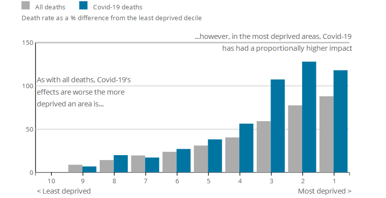
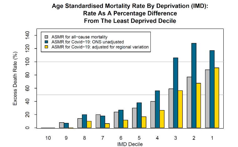
However, the source article for this data also indicated that infection and death rates in London were more than twice those of other regions. London also has a disproportionate number of deprived neighbourhoods (especially IMD deciles 2 and 3), relative to the country as a whole, and, if this is taken into account, then the impact of Covid-19 on deprived neighbourhoods is somewhat different from what the raw data in Figure 12 implies.

This is illustrated in Figure 13. The grey and blue bars are as in Figure 12. The gold bars adjust the blue bars for regional differences in Covid-19. The grey bars (all-cause mortality) and gold bars (Covid-19 mortality) can be directly compared against each other. We now see that Covid-19 mortality is very similar to all-cause mortality for deciles 1, 2, 3 and 10, the three most deprived and the least deprived areas, respectively. However, Covid-19 mortality in deciles 4 to 9 is about 10 to 15% lower than we would anticipate if Covid-19 mortality had the same degree of proportionality to all-cause mortality for these deciles as deciles 1, 2, 3 and 10. In other words, once we control for regional differences in mortality rates, Covid-19 deaths in both the most and least deprived groups are in proportion to the all-cause mortality of these groups.

In line with equation (1), the socio-economic analysis suggests a possible way of linking Covid-19 mortality with frailty for IMD sub-group i at age x: Covid mortality rate(i, x) = All-cause mortality rate(i, x) × Infection rate(i, x) × Relative frailty(i, x). If the product of the Infection rate(i, x) and Relative frailty(i, x) is constant (i.e., age independent) for each sub-group i, then the Sub-group Proportionality Hypothesis holds. The formal specification of the Sub-group Proportionality Hypothesis states that the product of sub-group i Infection rate(i, x) and Relative frailty(i, x) is constant (i.e., age independent), from which it follows that the Covid-19 mortality rate is proportional to all-cause mortality rate in a normal non-Covid year.

7. Observable Consequences of Accelerated Deaths Lessons from the Pattern of Deaths from Previous Respiratory Diseases

Everything else being equal, the ADM will predict higher death rates during the pandemic, followed by lower death rates after the pandemic due to anti-selection, before gradually reverting to previously predicted levels of mortality. This type of pattern in past mortality rates has been observed for respiratory diseases. Figure 14 shows death rates for respiratory diseases only (i.e., not all-cause mortality) by gender, age group and deprivation over the period 2001-2016. We can see clearly synchronized patterns over the years 2013, 2014 and 2015: a peak followed by a dip followed by another peak. This pattern is consistent with the 2012-13 influenza epidemic accelerating the deaths of people with chronic respiratory disease in 2013. This was followed by a dip in 2014 when there were fewer people with chronic respiratory diseases than normal, in combination with it being a quiet year for influenza.

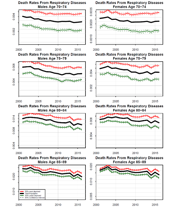
Also notable in the data is the fact that the pattern is strongest in the 85-89 age group, of similar magnitude for males and females, and weakens as we move to younger age groups. There are two potential reasons for the weakening signal at younger ages. First, it might simply be that there were many fewer accelerated deaths at younger ages. Second, the reach parameter might vary with age, with a longer reach at young ages and a short reach (e.g. ρ(x) = 1, say) at high ages, with many people dying in the same year.

We conclude that useful lessons about the potential pattern of accelerated deaths from Covid-19 can be drawn from examining deaths from respiratory diseases, especially at different age ranges.

8. Lessons from Past Seasonal Influenza Epidemics

Even before the Covid-19 pandemic, researchers had been paying a good deal of attention to weekly mortality registrations from the ONS and their potential impacts on mortality projections. These weekly returns are characterized by predictable seasonal fluctuations (with generally higher death rates in winter) and unpredictable influenza epidemics. Flu epidemics typically begin to emerge in December, but their precise timing is uncertain and their magnitude even more so. The ONS regularly publish weekly data by gender and age group, and, periodically, further subdivisions by IMD decile. A snapshot of these data for the 75-84 age group is presented in Figure 15. Deaths per 100,000 have been plotted on a log scale to emphasize the fact that the magnitudes of both predictable annual seasonal fluctuations and unpredictable flu epidemics do not depend significantly on either deprivation or gender.

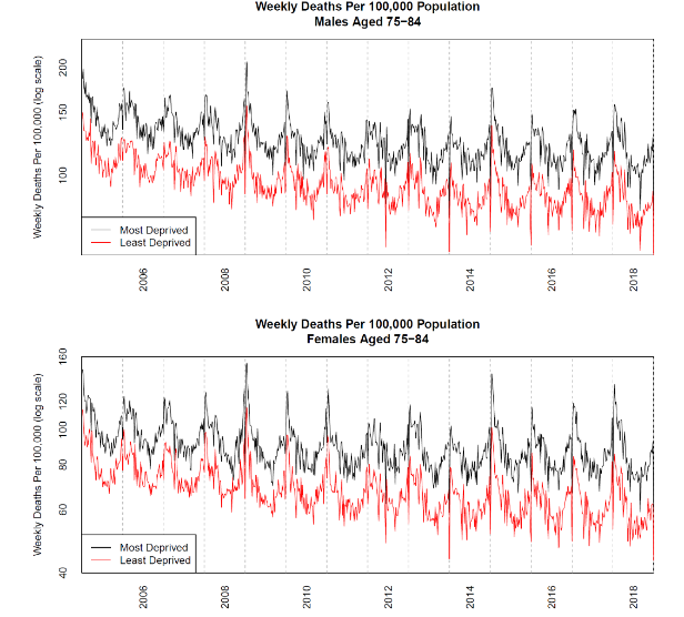
We conclude that it is possible to draw useful lessons about volatility spikes in Covid-19 deaths from examining past seasonal flu epidemics. However, there is an important difference. Whereas the spikes in seasonal flu increase with age, our finding that Covid-19 death rates are approximately proportional to all-cause mortality suggests that any spike in Covid-19 mortality in percentage terms would be similar across all age ranges.

9. Indirect Impacts of the Covid-19 Pandemic

The previous sections, and the ADM itself, assume that mortality rates for survivors revert to previous levels of mortality with no change to the annual mortality improvement rate. There are a number of reasons why this might not turn out to be the case, although, at present, none can be reliably or fully quantified:

• Some of those who have recovered from Covid-19 might carry forward some degree of impairment, possibly temporary, but also possibly long term. For example, a post-mortem study on patients who succumbed to the virus found that many experienced extensive kidney failure, while hospitals in Wuhan and New York City are treating many surviving Covid-19 patients for kidney failure. Similarly, liver function has failed to return to normal with many Covid-19 patients. Other examples include Covid-19 survivors developing sepsis or experiencing strokes, despite some being young and having only mild symptoms. Hard and extensive data on the numbers of impaired survivors is scarce at present. However, if impairments are more widespread (covering many more people than just intensive care survivors) and these do shorten life expectancies, then our model will need to be modified to treat those with impairments differently from other survivors.
• Delays in the treatment of non-Covid-19 patients because the health system cut back its non-essential services in order to redirect resources to deal with the pandemic and because diagnosis for other potentially serious illnesses. For example, thousands of cancers failed to be diagnosed every week because patients were not going to their doctor. Cancer Research UK reported that referrals by doctors for urgent hospital appointments fell by 75% ‒ equivalent to 2,300 cases per week. Another 400 cancers a week were missed because 200,000 weekly screenings for breast, cervical, lung and bowel cancer were suspended during the lockdown. A study from University College London (UCL) and the Health Data Research Hub for Cancer (DATA-CAN) predicted that up to 18,000 more people could die from cancer over the following year in England because of the impact of Covid-19.
• Self-isolation during lockdown and the economic recession that followed the ending of lockdown might have consequences for medium and long-term mortality:
  • Some of those who found themselves furloughed as a result of the lockdown increased their alcohol and drug consumption.
  • If the economy falls into recession for an extended period leading to long-term unemployment and/or more jobs are automated in response to the pandemic, this can result in deaths of despair.
  • The long-term impact of the economic downturn might reduce spending on medical and pharmaceutical research, causing a reduction in long-term future mortality improvements.
  • The pandemic might cause general medical advances to stall for a number of years as resources are redirected to finding a vaccine and treatments for Covid-19.
  • On the positive side, the behavioural changes required by lockdown ‒ such as social distancing, wearing face masks in public, and reduced automobile usage ‒ might have health benefits if these changes are adopted long term.
  • Similarly, the Covid-19 pandemic might also speed up the search for treatments that delay ageing, one of the primary factors that make people more susceptible to the virus.

10. Discussion

To investigate the impact of Covid-19 on higher-age mortality, we developed a simple decreasing exponential model of accelerated deaths (compared with scheduled deaths) that depends on two parameters: an amplitude (or impact) parameter which measures the number of Covid-19 deaths as a proportion of expected deaths in the next year due to all causes at the same age; and a reach parameter which measures the expected remaining years of life lost (i.e., remaining life expectancy) by those who die immediately from Covid-19.

We showed that, for plausible values of these two parameters, some of those who died from coronavirus would have died anyway in the relatively near future due to the presence of certain co-morbidities that Covid-19 fatally impacts, in particular, ischaemic heart diseases, dementia and Alzheimer’s disease, respiratory diseases, influenza and pneumonia, and diabetes. We also showed that the increase in life expectancy of survivors is likely to be very modest, around 0.2% at age 65. This implies that the impact of anti-selection on future life expectancies is negligible.

We noted that the model could be improved if we allowed the amplitude parameter to be a logistic function of age instead of being constant at all ages. With an appropriate parametrization of the logistic function, the model provided an excellent fit for Covid-19 deaths for England & Wales (EW). In terms of socio-economic differences in mortality, we argued that we needed to be careful about interpreting the data. Raw data from EW appears to suggest that members of more deprived socio-economic groups are more likely to contract and die from Covid-19 than those from less deprived groups. However, the raw data is biased by regional variations in Covid-19 mortality, in particular London which has much higher Covid-19 mortality and also a disproportionate number of deprived neighbourhoods relative to the rest of the EW.

Once this is taken into account, IMD (Index of Multiple Deprivation) data indicated that Covid-19 mortality is proportional to all-cause mortality for both the least deprived and most deprived groups. But it is 10 to 15% lower than we would anticipate for the middle-ranking deprivation groups, suggesting that these groups were better able to reduce their chances of contracting Covid-19 by, for example, working from home during the height of the pandemic.

The Accelerated Deaths Model could be used to predict that death rates will be lower in future years due to anti-selection, before gradually reverting to previously predicted levels of mortality. Peak mortality will depend primarily on the amplitude at various ages, while the size of the subsequent dip will depend more on the reach parameter. Identifying these effects in the data will, though, be complicated by the fact that each year in the future will have its own randomness, as well as seasonal influenza.

11. Conclusion

The Accelerated Deaths Model we have developed in this study is a very simple model for predicting post-pandemic mortality, especially at higher ages. The model is built on the observation that Covid-19 mortality in adults appears to be proportional to all-cause mortality. This is then extended to account for the observation that with respiratory diseases, there can be spikes in mortality in one year which are reversed in the following year, so that if Covid-19 behaves in a similar way, deaths are accelerated over scheduled deaths for a period of time before returning to normal. The parameter values for the model developed in this study were based on little more than educated guesswork of the kind that researchers would need to make at the start of any novel pandemic but these can be easily modified in the light of experience in order to calibrate the ex-post version of the ADM. Similarly, the model itself can also be modified or changed in due course. The model can also be adapted to match the experience of other countries.

However, the challenge is to calibrate an ex-ante version of the ADM suitable for a future pandemic. Suppose that we can assume that the Proportionality Hypothesis will hold. We would then need to make assumptions about the likely scale of the pandemic which is essentially an assumption about the amplitude parameter and also about the reach. Suppose that we can base the estimate of the reach parameter on the experience of a previous pandemic, such as Covid-19. Then the key task is to predict the scale of the pandemic. To do this, we would need to develop the magnitudes of which are measured on the Saffir-Simpson Hurricane Wind Scale with ratings between 1 (very dangerous winds will produce some damage, with speeds of 119-153 km/h) to 5 (catastrophic damage will occur, with speeds above 252 km/h); satellites are used predict the rating of each hurricane, which can be revised as the hurricane progresses and eventually peters out. We would need something similar for a future pandemic.

Recent developments in big data and sentiment analysis might be helpful in improving early trend detection, as the following examples indicate: Google Flu Trends and studies showing that sentiment analysis can predict outbreaks in real time, by processing news, or assessing individual risks, like 30-day mortality in sepsis patients, by analyzing unstructured text data from nursing notes.

Conflict of Interest:

None.

Funding Statement:

None.

Acknowledgements:

We would like to thank the participants at the numerous seminars we gave for their very helpful and constructive comments.

References:

• Banerjee, A., Pasea, L., Harris, S., Gonzalez-Izquierdo, A., Torralbo, A., Shallcross, L., Noursadeghi, M., Pillay, D., Sebire, N., Holmes, C, Pagel, C., Wong, W.K., Langenberg, C., Williams, B., Denaxas, S., Hemingway, H. (2020) Estimating excess 1-year mortality associated with the COVID-19 pandemic according to underlying conditions and age: A population-based cohort study. Lancet, 395:1715-1725. DOI: 10.1016/S0140-6736(20)30854-0.
• Bhaskaran, K., Rentsch, C. T., Hickman, G, Hulme, W. J., Schultze. A., Curtis, H.J, Wing, K., Warren-Gash, C., Tomlinson, L., Bates, C. J., Mathur, R., MacKenna, B., Mahalingasivam, V., Wong, A., Walker, A. J., Morton, C. E., Grint, D., Mehrkar, A., Eggo, R. M., Inglesby, P., Douglas, I. J., McDonald, H. I., Cockburn, J., Williamson, E. J., Evans, D., Parry, J., Hester, F., Harper, S., Evans, S. J. W., Bacon, S., Smeeth, L., and Goldacre, B. (2022) Overall and cause-specific hospitalisation and death after Covid-19 hospitalisation in England: A cohort study using linked primary care, secondary care, and death registration data in the OpenSAFELY platform. PLoS Med 19(1): e1003871. DOI: doi.org/10.1371/journal.pmed.1003871
• Cairns, A.J.G., Blake, D., Kessler, A., Kessler, M., Proportionality Hypothesis. European Actuarial Journal. DOI: doi.org/10.1007/s13385-024-00400-9
• Cairns, A.J.G., Wen, J., and Kleinow, T. (2024) Drivers of mortality: Risk factors and inequality. Journal of the Royal Statistical Society (Series A), 187: 989-1012
• (2022) The future evolution of the mortality acceleration due to the COVID-19: The Charlson Comorbidity Index in stochastic setting. Frontiers in Cardiovascular Medicine, 9. DOI: 10.3389/fcvm.2022.938086
• Case, A. and Deaton, A. (2015) Rising morbidity and mortality in midlife among white non-Hispanic Americans in the 21st century. Woodrow Wilson School of Public and International Affairs and Department of Economics, Princeton University, Princeton, NJ 08544.
• Case, A. and Deaton, A. (2017) Mortality and morbidity in the 21st century. Brookings Papers on Economic Activity, Spring: 397-476.
• Continuous Mortality Investigation (2019) Regular monitoring of England & Wales. CMI Working Paper 111.
• Docherty, A.B., Harrison, E. M., Green, C. A., Hardwick, H. E., Pius, R., Norman, L., Holden, K. A., Read, J. M., Dondelinger, F., Carson, G., Merson, L., Lee, J., Plotkin, D., Sigfrid, L., Halpin, S., Jackson, C., Gamble, C., Horby, P. W., Nguyen-Van-Tam, J. S., Dunning, J., Openshaw, P. J. M., Baillie, J. K., and Semple, M. G. (2020) Features of 16,749 hospitalized UK patients with COVID-19 using the ISARIC WHO Clinical Characterisation Protocol. MedArchiv Preprint, 28 April. DOI: doi.org/10.1101/2020.04.23.20076042
• Ferguson, N. M., Laydon, D., Nedjati-Gilani, G., Imai, N., Ainslie, K., Baguelin, M., Bhatia, S., Boonyasiri, A., Cucunubá, Z., Cuomo-Dannenburg, G., Dighe, A., Dorigatti, I., Fu, H., Gaythorpe, K., Green, W., Hamlet, A., Hinsley, W., Okell, L. C., van Elsland, C., Thompson, H., Verity, R., Volz, E., Wang, H., Wang, Y., Walker, P. G. T., Walters, C., Winskill, P., Whittaker, C., Donnelly, C. A., Riley, S., and Ghani, A. C. (2020) Report 9: Impact of non-pharmaceutical interventions (NPIs) to reduce COVID-19 mortality and healthcare demand. Imperial College Covid-19 Response Team, 16 March; https://spiral.imperial.ac.uk:8443/bitstream/10044/1/77482/14/2020-03-16-COVID19-Report-9.pdf
• Gompertz, B. (1825) On the nature of the function expressive of the law of human mortality, and on a new mode of determining the value of life contingencies. Philosophical Transactions of the Royal Society of London, 115: 513-585.
• Hanlon, P., Chadwick, F., Shah, A., Wood, R., Minton, J., McCartney, G., Fischbacher, C., Mair, F.S., Husmeier, D., Matthiopoulos, J., and McAllister, D.A., (2020) COVID-19 exploring the implications of long-term condition type and extent of multimorbidity on years of life lost: a modelling study. Wellcome Open Res, 5:75; https://wellcomeopenresearch.org/articles/5-75
• Krueger, A. B. (2017) Where have all the workers gone? An inquiry into the decline of the U.S. labor force participation rate. Brookings Papers on Economic Activity, Fall, 2017(2): 1-87. DOI:10.1353/eca.2017.0012
• Luo, O., O’Connell, D.L., Yu, X.Q., Kahn, C., Caruana, M., Pesola, F., Sasieni, P., Grogan, P.B., Aranda, S., Cabasag, C.J., Soerjomataram, I., Steinberg, J., and Canfell, K. (2022) Cancer incidence and mortality in Australia from 2020 to 2044 and an exploratory analysis of the potential effect of treatment delays during the Covid-19 pandemic: A statistical modelling study. Lancet Public Health, 7: e537-48.
• Mäki N., and Martikainen P. (2012) A register-based study on excess suicide mortality among unemployed men and women during different levels of unemployment in Finland. Journal of Epidemiology and Community Health, 66: 302-307; https://jech.bmj.com/content/66/4/302.long
• Reeves, A., McKee, M., Gunnell, D., Chang, S.-S., Basu, S., Barr, B., Stuckler, D. (2015) Economic shocks, resilience, and male suicides in the Great Recession: Cross-national analysis of 20 EU countries. European Journal of Public Health, 25(3): 404-409. DOI: doi.org/10.1093/eurpub/cku168
• Stuckler, D., Basu, S., Suhrcke, M., Coutts, A., and McKee, M. (2009) The public health effect of economic crises and alternative policy responses in Europe: An empirical analysis. Lancet, 374(9686):315-323. DOI: doi.org/10.1016/S0140-6736(09)61124-7
• Wu, D., Shu, T., Yang, X., Song, J.-X., Zhang, M., Yao, C., Liu, W., Huang, M., Yu, Y., Yang, Q., Zhu, T., Xu, J., Mu, J., Wang, Y., Wang, H., Tang, T., Ren, Y., Wu, Y., Lin, S.-H., Qiu, Y., Zhang, D.-Y., Shang, Y., and Zhou, X. (2020) Plasma metabolomic and lipidomic alterations associated with Covid-19, Wuhan Institute of Virology, 7 April; https://www.medrxiv.org/content/10.1101/2020.04.05.20053819v3.full.pdf.
• Yang, H.-C., Fogo, A. B., Nie. X., and Zhang, C. (2020) Renal histopathological analysis of 26 postmortem findings of patients with Covid-19 in China. Kidney International; https://www.kidney-international.org/article/S0085-2538(20)30369-0/fulltext.
• Zhou, F., Yu, T., Du, R., Fan, G., Liu, Y., Liu, Z., Xiang, J., Wang, Y., Song, B., Gu, X., Guan, L., Wei, Y., Li, H., Wu, X., Xu, J., Tu, S., Zhang, Y., Chen, H., and Cao, B. (2020) Clinical course and risk factors for mortality of adult inpatients with Covid-19 in Wuhan, China: A retrospective cohort study. Lancet, 28 March, 95(10229):1054-1062. DOI: 10.1016/S0140-6736(20)30566-3.

Data

• England & Wales, ONS: Deaths registered weekly in England and Wales, provisional; https://www.ons.gov.uk/peoplepopulationandcommunity/birthsdeathsandmarriages/deaths/datasets/weeklyprovisionalfiguresondeathsregisteredinenglandandwales/2020
• US, CDC: Weekly Updates by Select Demographic and Geographic characteristics; https://www.cdc.gov/nchs/nvss/vsrr/covid_weekly/

Appendix

We describe here a formal version of Equation (1). We consider a single individual aged x who has been infected at time 0, and then scale the cumulative Covid-19 death rate by the proportion of the age cohort infected. Define:

• μA(x) = death rate at age x from all causes in the absence of Covid-19
• μC(s, x) = death rate at time s and at age x from Covid-19 (assuming that the individual has been infected at time 0).

For simplicity in this Appendix, we will assume that μA(x) is constant over the next year (although in reality it is slowly rising), while, in contrast, μC(s, x) takes the shape of a short-lived, bell-shaped curve. Over the time interval [0, T], the cumulative death rates from the two sources are μA(x)T and ∫ μC(s, x)ds from 0 to T. Because the risk of dying from Covid-19 is short lived, the latter tends to a constant MC(x) as T tends to infinity, with convergence after only 4 or 5 weeks, say. Thus, over a given time period T (greater than 5 weeks, say), we can define Relative frailty, ω(x) = MC(x)/(μA(x)T). Note that this does mean that the value of relative frailty depends on the time horizon T.

“`