Evaluation of infectious diseases control using an individual model under the test-trace-isolate program

Yue Deng^1, Mingjing Li^1, Jiaqin Tan^2, Jinzhi Lei³

1. School of Software, Tiangong University, Tianjin, 300387, China
2. School of Computer Science and Technology, Tiangong University, Tianjin, 300387, China
3. School of Mathematical Sciences, Center for Applied Mathematics, Tiangong University, Tianjin, 300387, China

* [email protected]

OPEN ACCESS

PUBLISHED: 30 November 2024

CITATION: Deng, Y., Li, M., et al., 2024. Evaluation of infectious diseases control using an individual model under the test-trace-isolate program. Medical Research Archives, [online] 12(11). https://doi.org/10.18103/mra.v12i11.5987

COPYRIGHT © 2024 European Society of Medicine. This is an open-access article distributed under the terms of the Creative Commons Attribution License, which permits unrestricted use, distribution, and reproduction in any medium, provided the original author and source are credited.

DOI https://doi.org/10.18103/mra.v12i11.5987

ISSN 2375-1924

Abstract

The global public health situation is constantly threatened by infectious diseases. To effectively control the spread of these diseases, it is crucial to quickly disrupt the transmission pathways of the pathogens. During the COVID-19 pandemic, testing, tracing, and isolation programs effectively responded to disease outbreaks in some areas but have largely failed in many other countries. This study presents a computational model to evaluate the effectiveness of various prevention and control measures in managing epidemic transmission dynamics. The model utilizes an individual-based model and dynamic close-contact networks to simulate the spread of infectious diseases. By considering the dynamic contact network formed by different individuals and their activities in various social environments, the model can track the spread of the disease and changes in the infection status of each individual through simulation. Using COVID-19 as an example, the model simulations demonstrate that infections increase rapidly after a local outbreak without preventive measures, quickly reach a peak of daily new infections. However, implementing test-trace-isolate measures significantly decreases the scale of infections and the number of daily new cases. Further stringent preventive measures to reduce individual contact are required to achieve the goal of zero infections. The results emphasize the importance of early detection and isolation in curbing the spread of the virus. The model established in this study can be used to evaluate and optimize prevention and control measures to achieve the goal of zero infections.

Keywords: dynamic contact network; mask wearing rate; vaccination rate; individual-based model

Introduction

The COVID-19 pandemic has had a serious impact on global public health and the economy, highlighting the importance of a comprehensive evaluation of disease prevention measures and control strategies. By quantitatively evaluating the different prevention and control measures employed by various countries during infectious disease outbreaks, we can provide valuable insights for scientifically managing potential future outbreaks. Programs of testing, contact tracing, and isolation have successfully mitigated the spread of COVID-19 in countries like China, Korea, and Singapore, but have largely failed in many other regions. To promote more precise and effective epidemic prevention and control, it is necessary to conduct quantitative research on epidemic transmission dynamics under different prevention and control strategies.

Due to the uncertainties surrounding COVID-19, predictive mathematical models are crucial for forecasting the likely outcomes of disease outbreaks, informing healthcare needs, and minimizing the impact on people’s lives and economies. Previous studies have proposed various mathematical models to study the dynamic process of infectious diseases, offering valuable insights for predicting epidemic trends. However, many traditional infectious disease dynamic models assume a uniformly distributed population and use the mean-field assumption to simulate virus transmission. The assumption does not align with the reality that COVID-19 spreads through close-contact networks, which change with daily individual activities. Therefore, the close-contact relationships between individuals are dynamic and cannot be accurately described by the mean-field assumption.

Some studies have developed individual-based models to simulate the transmission dynamics of COVID-19 by focusing on individual-to-individual contacts and heterogeneous responses among individuals. Individual-based models allow us to track the process of disease outbreaks and simulate varied responses and control measures for different individuals, providing a valuable technique for evaluating the influence of the test-trace-isolate programs.

This paper introduces an individual-based model designed to simulate how individuals moving within communities and different environments influence epidemic transmission dynamics. The model considers individual activities and changes in disease status to simulate the dynamic process of infectious diseases following a local epidemic outbreak. We applied the model to evaluate the impact of different prevention and control measures on the epidemic’s evolution. Specifically, the model includes measures such as testing, tracing, and isolation to quantitatively assess their effects on controlling the spread of the epidemic. This model can digitally reconstruct the regional disease transmission process and predict the epidemic’s evolution under different prevention and control measures, thus providing guidance for strategic decision-making in disease prevention and control. The paper uses COVID-19 as a case study to introduce the model and calculate the relevant parameters. This model can also be applied to infectious diseases with similar transmission characteristics.

Methods

In this paper, we established a model to simulate the spread of infectious diseases after a local outbreak. The local area comprises functional compartments such as residential communities, workplaces, schools, and other settings. A discrete computational model based on individual activities was developed to simulate both individual activities and disease transmission within the area. The model mainly consists of two parts. One part simulates the contact situation of all individuals, known as the dynamic contact network; the other simulates changes in the infectious disease status of each individual, known as the individual-based model. While the model uses COVID-19 as an example, its structure can be applied to other similar respiratory infectious diseases. Detailed descriptions of the model are provided below.

INDIVIDUAL-BASED MODEL

The individual-based model was developed with reference to existing models. The model was designed to simulate the epidemic dynamics in a local area, such as a city containing at most N individuals. All individuals form a dynamic contact network through close contacts, with each individual represented as a node in the network. The epidemic status of each node can be categorized as vacancy (V), susceptible (S), infectious (I) (including latent, asymptomatic, and symptomatic infectious), confirmed (H), quarantined (Q), recovered (R), and death (D) according to the status change of the corresponding individual. The vacancy indicates no individual at the node (for example, if the corresponding individual has migrated or died). Each node, except for vacancies, represents an individual who dynamically changes between six statuses according to the basic assumptions of the susceptible-infectious-confirmed-quarantined-recovered-death (SIHQRD) model.

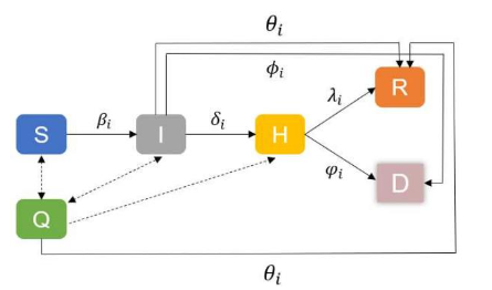
In the SIHQRD model, a susceptible individual (S) becomes infectious (I) with an infection rate βi(t) after contact with an infectious individual. The situations of latent, asymptomatic infectious, and symptomatic infectious are not distinguished in this model, but different infection stages are distinguished by the variance in their infection rates and confirmed rates. Infectious individuals (I) become confirmed (H) with a rate δi(t). The confirmed rate is related to the duration of infection and the frequency of nucleic acid testing (NAT) for infectious individuals. Moreover, we assumed that confirmed cases were hospitalized immediately, thus no longer contacting susceptible individuals. When an infectious individual is confirmed, their close contacts are tracked through the contact network of the confirmed case. Following the test-trace-isolate program, close contacts of the confirmed case are isolated and become quarantined (Q). Quarantined persons cannot contact others and are tested for nucleic acid during the isolation period. Individuals confirmed during the quarantine period enter the confirmed status; otherwise, they return to their status before isolation (susceptible(S), infectious (I), or recovered (R)) after the isolation period. Infectious individuals may recover with a recovered rate θi(t). Confirmed cases (H) may either recover with a rate λi(t) or death (D) with a rate ϕi(t).

The model highlights individual differences and stochastic dynamic changes and considers changes in the total number of individuals by introducing.

DYNAMIC CONTACT NETWORK

The dynamic contact network was divided into family contacts and public contact networks, such as workplaces, schools, and other public places, according to contact relationships between different individuals. Each individual can simultaneously belong to the family contact network and different public network modules. The contact network matrix T(t) represents the network formed by N individuals through contact relationships. The matrix T(t) can vary over time due to changes in contact relationships. The matrix T(t) is an N × N matrix, with elements defined as follows:

To track the close contact relationship between individuals, we introduced S(t) as the effective contact matrix between individuals. The two individuals are considered effective contacts at time t if they have been in close contact within the effective contact time ET (in days) before the current moment t. The element Sij(t) indicates whether individual i and individual j have had close contact during the past effective contact period. We set Sij(t) = 0 if individual i and the individual j have had no contact during the effective contact period, and Sij(t) > 0 represents the days from the current moment of the last close contact between individuals i and j. For instance, Sij(t) = k means that i and j have close contact k days earlier. We set Sij(t) = 0 if Sij(t) exceeds the maximum value of the effective contact time ET. Hence, the matrix Sij(t) is defined as follows:

It is easy to see that S(t) is a symmetry matrix. The effective contact matrix Sij(t) is updated daily according to the contact relationship Tij(t), and the matrix Sij(t+1) is given as follows:

When constructing the contact network matrix, N individuals were first divided into family units, with each family unit containing 1 to 6 individuals who form close contact relationships. Next, each family member was randomly assigned to different public networks. The two networks were updated alternately according to individual activities. Usually, the contact relationship between family members does not vary over time. To describe the close contact relationship of the public networks, we utilized a small-world network to approximate the close contact relationship in each public network instead of tracking the activation of each individual. Different contact properties of public networks can be represented by their small-world network parameters. The statistical properties of social networks have been extensively studied, and small-world networks can effectively describe the features of social networks and simulated the contact networks. Hence, using a small-world network to describe contact relationships between individuals in the public network is appropriate. The parameters of the small-world network in the current study are listed in Table A.1 in the Appendix.

The contact network matrix Tij(t) includes different network modules of family contacts and public networks. The individual contact relationships of the family network are fully connected, while the individual contact relationships in each public network are updated according to the small-world network. Moreover, if an individual is quarantined, confirmed, or dead, the contact relationships between that individual and others are eliminated and no longer updated. In this study, eight public networks were considered, including three type-I networks with mostly fixed individuals, such as workplaces, schools, kindergartens, and buildings, and five type-II networks with relatively mobile individuals, such as restaurants, marketplaces, buses, and subways. The network structure parameters for different public networks were varied. In type-I networks, individuals were mostly fixed, and the contact relationship and network parameters remained unchanged. However, the infection status of each individual within these networks could vary over time (e.g., isolation, confirmed, or dead). In contrast, type-II networks and their contact networks changed daily, forming a dynamic contact network relationship. Different network parameters were set in our model to represent the unique features of each network, including individual update probabilities, as shown in Table A.2 in the Appendix.

STATE TRANSITION OF INDIVIDUALS

To model the transition of individuals to an infectious state, we need to formulate the transition rates between different statuses.

INFECTION

During infectious disease transmission, an infected individual contacts a susceptible individual and transmits the virus to them. Let IRi,j represent the infection probability in one day when a susceptible individual i comes into contact with an infectious individual j. Then, the probability that susceptible individual i is infected in one day through close contacts is given by:

Here, N(i) represents all close contacts of the individual i. If susceptible individual i is vaccinated, the infection rate may be reduced. Let Vi represent the efficiency of the vaccine; then the infection probability should be modified as:

Here, 0 ≤ Vi < 1 represents the reduction in the infection probability, with Vi = 0 indicating no vaccination. In our model simulation, we used the following values:

The infection probability between a susceptible individual i and an infected individual j can be influenced by their mask-wearing situations and the infectiousness of the infected individual j. Mask-wearing reduces the transmission of respiratory infectious diseases. To account for the effect of mask-wearing, let Mi,j represent the reduction factor of the infection rate due to different mask-wearing situations of the susceptible i and the infected j. We set the following values in our model simulation:

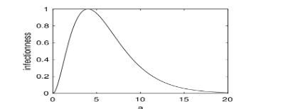
The SARS-CoV-2 viral load varies after initial exposure, typically leading to symptom development within 5-6 days. Consequently, the infectiousness of the infected individual j changes depending on the time after initial exposure, referred to as the infection age a. To account for this variance, we introduced a function f(a) to describe the dependence of infectiousness on the infection age a:

Here, a is the time since the initial exposure (days). Figure 2 shows the plot of f(a), which trends similarly to the SARS-CoV-2 viral load and reaches a maximum value of 1 at a = 4.

Based on the effective factor Mi,j and the infectiousness function f(a), the infection probability IRi,j is expressed as where IR is the maximum infection probability, and aj is the infection age of the infected individual j. In our model simulations, we set IR = 0.9, referring to the Omicron SARS-CoV-2. This means that when a susceptible and an infected individual are in close contact without any prevention, the probability of infection is 90%. Each individual has a preference for wearing a mask every day, so the situation regarding mask-wearing can vary daily.

Equations (2.5) and (2.9) together provide the probability that a susceptible individual will be infected by close contact, taking into account the influences of vaccine protection, mask-wearing, and the temporal variation of infectiousness.

CONFIRMATION OF INFECTIOUS INDIVIDUALS

We assumed that an infected individual i is confirmed with a confirmation rate δi(t). Various clinical factors may affect a patient’s confirmation rate. However, in this model, we simplify the situation by assuming the confirmation rate only depends on the symptoms, which are associated with viral load, or the infectiousness f(ai). Thus, for simplicity, we assumed that the confirmation rate is proportional to the infectiousness:

where δ is the maximum confirmation rate. Once an individual is confirmed, they are hospitalized and lose all contact with others.

CLOSE CONTACT TRACING AND ISOLATION

When a confirmed case is identified, close contact tracing and isolation programs are immediately initiated. Previous studies have shown that these measures are crucial for breaking the transmission chain of the disease and preventing the spreading of the epidemic. Using the effective contact matrix S(t), we can determine the individuals who have been in close contact with an infected individual. For example, the close contacts of individual i at time t forms a subset Ci(t) = {i ≤ j ≤ N | Sij(t) > 0}. For each j ∈ Ci(t), we can further identify their close contacts, forming the secondary level contacts of the individual i. Under different control measures, first and secondary-level contacts may be isolated to block virus transmission. Once a confirmed case is identified, close contacts are traced and isolated. However, this process can be complex in reality, as it takes time to trace the close contacts, and identifying all contacts is usually challenging. In our model simulations, we introduced two parameters to represent the probabilities of finding the close and secondary-level contacts, respectively. For simplicity, we assumed that close contacts are isolated on the second day after the confirmed case is identified. Isolation typically lasts one or two weeks, depending on the control measures.

For isolated individuals, nucleic acid testing (NAT) is assumed to be performed on specified days after isolation. Those confirmed by NAT are hospitalized, and their close contacts are traced and isolated. Individuals who are not confirmed during the isolation period return to their normal lives.

RECOVERY OR DEATH

Each infected individual recovers at a rate θi(t). The recovery rate θi(t) is associated with the infection age ai since the initial exposure. The isolated infected individuals have the same recovery rate θi(t). Confirmed infected individuals who are hospitalized have a higher recovery rate λi(t). We simply assumed:

Patients with mild to moderate illness often have a high rate of self-recovery, while those with severe or clinical illness are more likely to be confirmed and hospitalized. Each infectious individual may die at a rate ϕ. Hospitalized patients have a lower death rate ϕ (ϕ < ϕ).

According to the WHO, the death rate of COVID-19 patients was approximately 2−3% in 2020 and decreased to 0.6−1.0% in 2024. However, since many COVID-19 infections recover without medical intervention, the actual death rate is likely lower than these reported figures.

NUMERICAL SCHEME

In numerical simulations, we update the infectious status of each individual and the contact network daily, following a stochastic simulation method based on changes in individual status. To simulate the impact of different prevention and control measures, we introduce daily variance in the system in accordance with these measures. A brief summary of the numerical scheme is given below:

Initialization: Initialize the system with the initial contact network and the initial infection status of each individual.

1. Initialize the nodes in the network, assigning either vacancies or individuals.
2. Initialized the contact network; assign each individual to a family network and a public network, and set the initial infection status of each individual.
3. Calculate the status transition rates for each individual.

Update: Update the infection status of each individual and the contact network daily.

1. Update the mask-wearing status of each individual according to their preference for wearing masks.
2. Update the dynamic contact network. Type-I networks contain fixed individuals, and their contact relationships may change daily based on the small-world network model. Type-II networks may include alterable individuals, with membership varying daily. The corresponding individuals and contact networks are updated to maintain a dynamic contact network.
3. Update the infection status of each individual based on the contact network and the infection status of others.
4. Update variables that dynamically change over time and may depend on control measures, such as mask-wearing rate, the number of new confirmed cases, the total number of confirmed cases, the number of new deaths, the total number of deaths, the number of close contacts, etc.

Simulation termination: Terminate the simulation when the simulation time is reached and save the epidemic dynamics generated by the model.

PARAMETER ESTIMATION

In this study, the model parameters were set with reference to the epidemic spread of COVID-19, particularly focusing on the Omicron variant. The parameters for the contact network and individual status are shown in Table A.2 and Table A.3 in the Appendix. Most parameters were estimated based on prior experience and adjusted to align with real-world epidemic data.

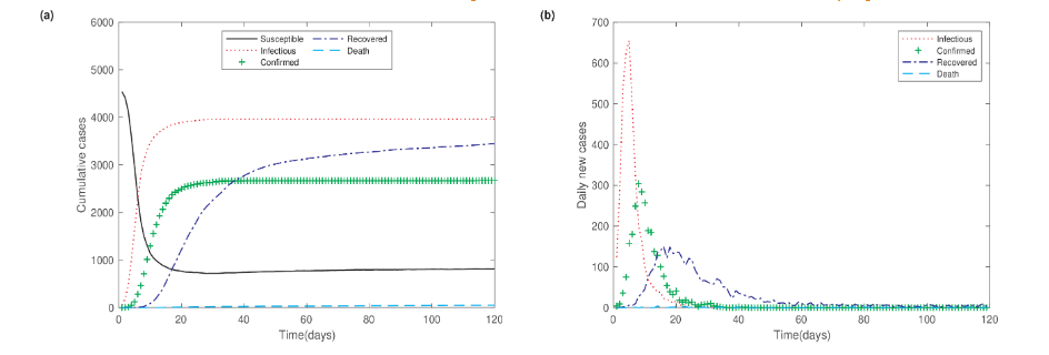
In model simulations, we set the total population size to N = 5000 and adjusted the model parameters to reflect the Omicron SARS-CoV-2 epidemic. Without prevention and control measures, the epidemic dynamics reach a stable state in 30 days, with approximately 80% individuals infected. The peak of new daily infections occurs one week after the outbreak begins.

Results

IMPACT OF WEARING MASKS ON THE EVOLUTION OF EPIDEMIC

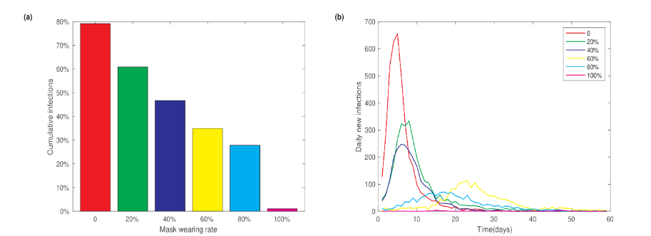
To examine the impact of mask-wearing on the epidemic size, we performed model simulations with varying mask-wearing rates. We fixed other parameters at their default values as listed in Table A.2 and Table A.3 and did not consider the measures of contact tracing and isolation. Figure 4a shows the dependence of the final cumulative infection fraction on the mask-wearing rates. The 0 mask-wearing rate corresponds to the scenario without any control measures, as shown in Figure 3. As the mask-wearing rate increased from 0 to 20%, 40%, 60%, and 80%, the cumulative infections decreased from 80% to 60%, 46%, 35% and 28%, respectively. If the mask-wearing rate increases to an extreme level of 100%, meaning that all individuals wear masks whenever they are in close contact, the cumulative infection fraction would reduce to an extremely low level of 1%. Additionally, increasing the mask-wearing rate significantly reduces daily new infections and postpones the time to reach the peak of daily new cases. These results highlight the importance of mask-wearing in preventing the spread of disease.

EFFECTS OF CLOSE CONTACT ISOLATION MEASURES

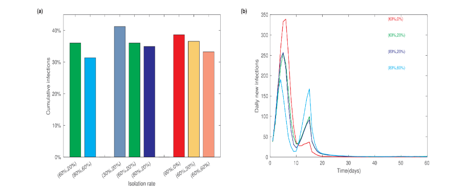
To evaluate the effectiveness of tracing and isolation, we varied the isolation rates for the first and the second-level close contacts and examined the final level of cumulative infections. When the isolation rates for the first and second-level close contacts were set at 60% and 20%, respectively, the final cumulative infection percentage decreased from 80% (in the absence of prevention measures) to 36%. The percentage further decreased to 31% when the isolation rates were increased to 80% for the first-level and 60% for the second-level contacts. If the second-level contact isolation rate was fixed at 20% and the first-level isolation rate was varied, the cumulative infections percentage increased to 41% when only 30% close contacts were isolated. However, there was no significant difference in the cumulative infection percentage when the isolation rate increased from 60% to 80%. We also fixed the first-level contact isolation rate at 60% and varied the second-level isolation rate at 0%, 30%, and 60%. The resulting cumulative infections were 39%, 37%, and 33%, respectively.

We also analyzed the dynamics of daily new infections under different isolation rates. Compared to the scenario without control measures, the application of tracing and isolation measures resulted in distinct dynamics of daily new infections. Figure 5b shows two peaks in the number of daily new infections. The first peak occurs at approximately one week, similar to the scenario without control measures, but with a lower maximum value of daily new infections. Interestingly, there is a second peak in the daily new infection numbers around two weeks after the disease outbreak. The magnitude of the second peak mainly depends on the second-level isolation rate, with higher rates resulting in a more pronounced second peak and a reduced first peak.

These results indicate that the tracing and isolation program can significantly reduce infection numbers. Second-level close contact isolation plays a role in shaping the daily dynamics of new infections.

IMPACT OF SOCIAL RESTRICTION CONTROL MEASURES

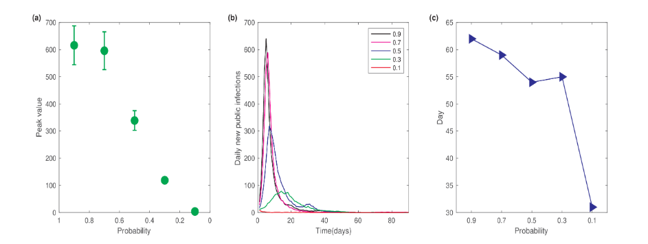
To evaluate the impact of social restrictions on epidemic dynamics, we varied the probability of individuals entering the public network. The public network represents public places where people congregate, forming dynamic contact networks. Figure 6a shows the dependence of the peak value of daily new infections on the probability of entering the public network. Here, we set the mask-wearing rate as 0, and no tracing or isolation measures were applied for close contacts. Hence, a probability of 1 represents the situation without control measures. As shown in Figure 6a, when the probability decreased from 0.7 to 0.5, the peak value of daily new infections significantly decreased from 600 to 339. The peak value further continued to decrease with lower probabilities of entering the public network. These results indicate that implementing social restrictions can effectively reduce the number of infections and help control the spread of the epidemic.

We further examined the influence of social restrictions on the time required to achieve zero new infections. To quantify this “zero clearing” time, we only considered new infections occurring within the public network. The epidemic was considered to have cleared if there were zero new public cases for five consecutive days. Figure 6b shows the temporal dynamics of daily new public infections for different probabilities of public network entry. The results indicated that as the probability decreased, both the peak value of daily new infections decreased, and the time to reach this peak was postponed. These findings suggest that decreasing the probability of entry into public networks can reduce the epidemic size and slow its spread. The dependence of the zero-clearing time on the public network entry probability is depicted in Figure 6c, showing that stricter restrictions on public networks result in a shorter zero clearing time.

INFLUENCE OF DYNAMIC CONTACT NETWORK STRUCTURE

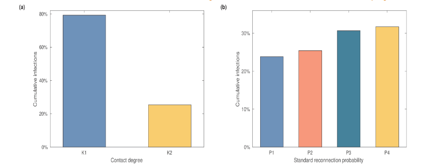
While social restrictions can effectively reduce the epidemic size and shorten the time to zero new infections, they may also cause significant inconvenience in daily life. Alternatively, reducing the number of contacts in public networks can help prevent the spread of the epidemic. To evaluate the effects of reducing public contacts, we adjusted the structure parameters (K, P) in defining the public contact networks. Here, the contact degree K refers to the average number of close contacts per individual, and P represents the reconnection probability.

First, we compared the results of two network structures with different parameter sets for K across the 8 public networks. The first network used values from the default parameters (K1), corresponding to the situation without control measures. In contrast, the second network assumed that social restrictions were implemented starting on the 15th day after the epidemic outbreak, leading to a reduction in the parameters K (K2). Model simulations showed that when the contact degree changed from K1 to K2, the fraction of cumulative infections decreased from 79% to 25%.

Next, we fixed the average contact degree at K2 and varied the reconnection probability P for different public subnetworks. The cumulative infection numbers are shown in Figure 7b. The cumulative number of infections increases with the standard reconnection probability. These results indicate that the structure of the close contact network in public settings significantly impacts the final epidemic size. Measures such as reducing the average contact degree and the standard reconnection probability can effectively prevent the spread of the epidemic.

INFLUENCE OF MULTIPLE CONTROL MEASURES

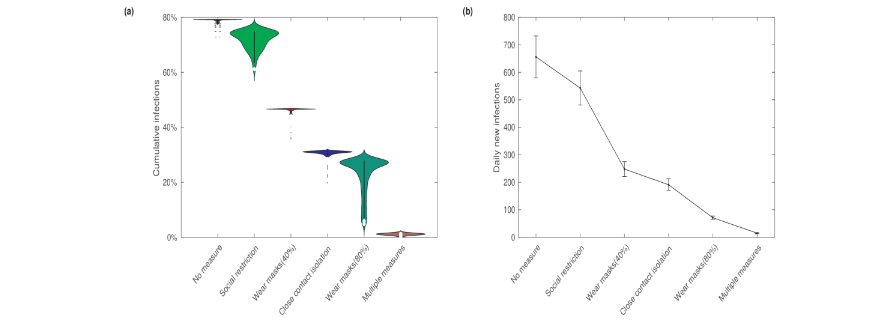
In the previous discussions, we examined different control measures individually. Now, we assess the effectiveness of implementing multiple measures in combination. The control measures we considered include close contact isolation, mask-wearing, and social restriction. We assumed the isolation rates for the first and the secondary-level close contacts to be 80% and 60%, respectively, a mask-wearing probability at either a low (40%) or a high (80%) level, and a public network entering probability of 0.8.

Figure 8 presents the fractions of the cumulative number of infections and the maximum daily new infections under various scenarios: no control measures, single control measures (close contact isolation, mask-wearing, social restriction), and the combination of multiple control measures. The results indicate that the fraction of the cumulative number of infections is the highest when no prevention and control measures are in place. Implementing social restrictions significantly reduces the cumulative infections. Similarly, close contact isolation and mask-wearing also notably reduce the cumulative infections. Notably, increasing the mask-wearing rate has a substantial impact on the epidemic, significantly lowering the cumulative number of infections. Furthermore, these measures have similar effects on both the cumulative number of infections and the maximum daily new infections.

Implementing multiple prevention and control measures simultaneously has the most significant and effective impact on the epidemic, reducing both the cumulative number of infections and the maximum daily new infections to very low levels.

Discussion

This study introduces an individual-based computational model with dynamic contact networks to simulate the transmission dynamics of local infectious disease outbreaks. Specifically, the model evaluates the impact of the test-trace-isolate program on the evolution of an epidemic by analyzing key indicators such as cumulative infection numbers, peak infection rates, and daily new infections under various prevention and control measures.

In the absence of any preventive interventions, the simulations show a rapid rise in infections following the emergence of a local outbreak. The peak in daily new infections typically occurs within approximately one week, underscoring the swift escalation of transmission in such scenarios. However, the introduction of the test-trace-isolate program markedly slows the rate of infectious spread, resulting in a substantial reduction in both the final epidemic size and the number of daily new cases. Specific measures—including reducing interpersonal contact, effectively tracing and isolating close contacts, and implementing broader social restrictions—demonstrated a significant impact on curbing the overall scale of the epidemic.

This model offers valuable quantitative insights into the effectiveness of preventive strategies against COVID-19, particularly in relation to more transmissible variants such as the Omicron strain. Beyond COVID-19, the framework developed here is adaptable for the evaluation of prevention and control measures for other infectious diseases, allowing for comparative assessments across different pathogen characteristics and epidemic settings. By simulating individual behaviors and network interactions, this approach can be expanded to incorporate diverse public health interventions, such as vaccination campaigns, population-level behavior modifications, and varying levels of public adherence to guidelines.

One notable feature of this study is its approximation of individual contact relationships within public networks using a small-world network model. While this offers a useful abstraction for modeling local interactions, it does not fully capture the complexity of real-world contact patterns. Real-life social networks are dynamic and heterogeneous, with varying degrees of clustering, multi-layered interactions, and shifts in contact rates over time due to behavioral, social, and policy-related changes. Accurately modeling these complex dynamics in future iterations remains a challenge, but is crucial for improving predictive power and precision in assessing outbreak responses.

Moreover, the model assumes a level of consistency in the effectiveness of interventions such as contact tracing and isolation. However, in real-world applications, these interventions are often hampered by factors such as delays in testing, incomplete tracing, non-compliance with isolation orders, and the varying availability of resources across different regions. Future modeling efforts should incorporate these real-world inefficiencies to provide more nuanced predictions and improve public health planning.

As infectious diseases continue to evolve, the next frontier in epidemic modeling will likely involve the integration of real-time data streams, such as mobile health data, geolocation tracking, and population mobility patterns. These data sources can help to more accurately simulate contact networks and adjust intervention strategies dynamically as new data emerge. Additionally, machine learning techniques could be employed to refine predictions and optimize the allocation of resources during an outbreak.

Conclusion

This study provides a robust framework for evaluating the effectiveness of the test-trace-isolate program and other non-pharmaceutical interventions in managing infectious disease outbreaks. While the model offers valuable insights, future efforts must focus on addressing the limitations associated with the complexity of human contact networks and real-world intervention constraints. Enhancing the fidelity of these models will play a critical role in improving public health responses to future pandemics, helping to mitigate their impact more effectively.

References

1. Y. Pei, E. Aruffo, E. Gatov, Y. Tan, Q. Li, N. Ogden, S. Collier, B. Nasri, I. Moyles, H. Zhu. School and community reopening during the COVID-19 pandemic: a mathematical modeling study, R Soc Open Sci 9 (2) (2022) 211883.
2. C. N. Ngonghala, E. Iboi, S. Eikenberry, M. Scotch, C. R. Macintyre, M. H. Bonds, A. B. Gumel. Mathematical assessment of the impact of non-pharmaceutical interventions on curtailing the 2019 novel coronavirus, Math Biosci 325 (2020) 108364 – 108364.
3. P. Yuan, Y. Tan, L. Yang, E. Aruffo, N. H. Ogden, G. Yang, H. Lu, Z. Lin, W. Lin, W. Ma, M. Fan, K. Wang, J. Shen, T. Chen, H. Zhu. Assessing the mechanism of citywide test-trace-isolate Zero-COVID policy and exit strategy of COVID-19 pandemic, Infect Dis Poverty 11 (1) (2022) 104.
4. The Lancet Digital Health, Contact tracing: digital health on the frontline, Lancet Digit Health 2 (11) (2020) e561.
5. D. Lewis. Why many countries failed at COVID contact-tracing-but some got it right, Nature 588 (7838) (2020) 384–387.
6. X. Wang, Z. Du, E. James, S. J. Fox, M. Lachmann, L. A. Meyers. D. Bhavnani, The effectiveness of COVID-19 testing and contact tracing in a US city. Proc Natl Acad Sci USA 119 (34) (2022) e220652119.
7. H. W. Hethcote. The mathematics of infectious diseases, SIAM Rev. 42 (2000) 599–653.
8. B. Tang, F. Xia, S. Tang, N. L. Bragazzi, Q. Li, X. Sun, J. Liang, Y. Xiao, J. Wu. The effectiveness of quarantine and isolation determine the trend of the COVID-19 epidemic in the final phase of the current outbreak in China, Int J Infect Dis 96 (2020) 636 – 647.
9. K. Chatterjee, K. Chatterjee, A. Kumar, S. Shankar. Healthcare impact of covid-19 epidemic in india: A stochastic mathematical model, Medical Journal, Armed Forces India 76 (2020) 147 – 155.
10. A. Bertozzi, E. Franco, G. O. Mohler, M. B. Short, D. Sledge. The challenges of modeling and forecasting the spread of covid-19, Proc Natl Acad Sci USA 117 (2020) 16732 – 16738.
11. F. Wu, X. Liang, J. Lei. Modelling COVID-19 epidemic with confirmed cases-driven contact tracing quarantine, Infect Dis Model 8 (2023) 415–426.
12. L. Yin, H. Zhang, Y. Li, K. Liu, T. Chen, W. Luo, S. Lai, Y. Li, X. Tang, L. Ning. Effectiveness of contact tracing, mask wearing and prompt testing on suppressing COVID-19 resurgences in megacities: An individual-based modelling study, Social Science Electronic Publishing (2021) doi: 10.2139/ssrn.3765491.
13. M. K. Chae, D. U. Hwang, K. Nah, W. S. Son. Evaluation of COVID-19 intervention policies in South Korea using the stochastic individual-based model, Sci Rep 13 (1) (2023) 18945.
14. C. Xu, Y. Pei, S. Liu, J. Lei. Effectiveness of non-pharmaceutical interventions against local transmission of COVID-19: An individual-based modelling study, Infect Dis Model 6 (2021) 848 – 858.
15. M. Ajelli, B. Gonçalves, D. Balcan, V. Colizza, A. Vespignani. Comparing large-scale computational approaches to epidemic modeling: Agent-based versus structured metapopulation models, BMC Infectious Diseases 10 (1) (2010) 1–13.
16. S. L. Chang, N. Harding, C. Zachreson, O. M. Cliff, M. Prokopenko, Modelling transmission and control of the COVID-19 pandemic in Australia, Nat Commun 11 (2020).
17. N. Masuda, N. Konno, K. Aihara, Transmission of severe acute respiratory syndrome in dynamical small-world networks, Phys Rev E 69 (3) (2004) 031917.
18. G. Hartvigsen, J. M. Dresch, A. L. Zielinski, A. J. Macula, C. C. Leary. Network structure, and vaccination strategy and effort interact to affect the dynamics of influenza epidemics, J Theor Biol 246 (2) (2007) 205–213.
19. M. H. Chua, W. Cheng, S. S. Goh, J. Kong, B. Li, J. Y. C. Lim, L. Mao, S. Wang, K. Xue, L. Yang, E. Ye, K. Zhang, W. C. D. Cheong, B. H. Tan, Z. Li, B. H. Tan, X. J. Loh. Face masks in the new COVID-19 normal: Materials, testing, and perspectives, Research (Wash D C) 2020(2020)7286735.doi:10.34133/2020/7286735.
20. K. Escandón, A. L. Rasmussen, I. I. Bogoch, E. J. Murray, K. Escandón, S. V. Popescu, J. Kindrachuk, COVID-19 false dichotomies and a comprehensive review of the evidence regarding public health, COVID-19 symptomatology, SARS-CoV-2 transmission, mask wearing, and reinfection, BMC Infect Dis 21 (1) (2021) 710. doi:10.1186/s12879-021-06357-4.
21. M. Liao, H. Liu, X. Wang, X. Hu, Y. Huang, X. Liu, K. Brenan, J. Mecha, M. Nirmalan, J. R. Lu, A technical review of face mask wearing in preventing respiratory COVID-19 transmission, Curr Opin Colloid Interface Sci 52 (2021) 101417. doi:10.1016/j.cocis.2021.101417.
22. S. A. Saint, D. A. Moscovitch, Effects of mask-wearing on social anxiety: an exploratory review, Anxiety Stress Coping 34 (5) (2021) 487-502.doi:10.1080/10615806.2021.1929936.
23. M. Cevik, K. Kuppalli, J. Kindrachuk, M. Peiris, Virology, transmission, and pathogenesis of SARS-CoV-2, BMJ 371 (2020).
24. J. Hellewell, S. Abbott, A. Gimma, N. I. Bosse, C. I. Jarvis, T. W. Russell, J. D. Munday, A. J. Kucharski, W. J. Edmunds, Centre for the Mathematical Modelling of Infectious Disease COVID-19 Working Group, S. Funk, R. M. Eggo, Feasibility of controlling COVID-19 outbreaks by isolation of cases and contacts, Lancet Global Health 8 (4) (2020) e488–e496.
25. E. L. Davis, T. C. D. Lucas, A. Borlase, T. M. Pollington, S. Abbott, D. Ayabina, T. Crellen, J. Hellewell, L. Pi, CMMID COVID-19 Working Group, G. F. Medley, T. D. Hollingsworth, P. Klepac, Contact tracing is an imperfect tool for controlling COVID-19 transmission and relies on population adherence, Nat Commun 12 (2021) 5412.
26. S. Contreras, J. Dehning, M. Loidolt, J. Zierenberg, F. P. Spitzner, J.-H. Urrea-Quintero, S. B. Mohr, M. Wilczek, M. Wibral, V. Priesemann, The challenges of containing SARS-CoV-2 via test-trace-and-isolate, Nat Commun 12 (1) (2021) 378.
27. P. Yuan, J. Li, E. Aruffo, E. Gatov, Q. Li, T. Zheng, N. H. Ogden, B. Sander, J. Heffernan, S. Collier, Y. Tan, J. Li, J. Arino, J. Bélair, J. Watmough, J. D. Kong, I. Moyles, H. Zhu, Efficacy of a “stay-at-home” policy on SARS-CoV-2 transmission in Toronto, Canada: a mathematical modelling study, CMAJ Open 10 (2) (2022) E367–E378.
28. W. H. Organization. Global excess deaths associated with covid-19 [online].
29. Z. Chen, X. Deng, L. Fang, K. Sun, Y. Wu, T. Che, J. Zou, J. Cai, H. Liu, Y. Wang, T. Wang, Y. Tian, N. Zheng, X. Yan, R. Sun, X. Xu, X. Zhou, S. Ge, Y. Liang, L. Yi, J. Yang, J. Zhang, M. Ajelli, H. Yu, Epidemiological characteristics and transmission dynamics of the outbreak caused by the SARS-CoV-2 Omicron variant in Shanghai, China: a descriptive study, Lancet Reg Health West Pac 29 (2022) 100592. doi:10.1101/2022.06.11.22276273.
30. P. Elliott, O. Eales, B. Bodinier, D. Tang, H. Wang, J. Jonnerby, D. Haw, J. Elliott, M. Whitaker, C. E. Walters, C. Atchison, P. J. Diggle, A. J. Page, A. J. Trotter, D. Ashby, W. Barclay, G. Taylor, H. Ward, A. Darzi, G. S. Cooke, M. Chadeau-Hyam, C. A. Donnelly, Dynamics of a national Omicron SARS-CoV-2 epidemic during January 2022 in England, Nat Commun 13 (1) (2022) 4500. doi:10.1038/s41467-022-32121-6.
31. O. Eales, L. de Oliveira Martins, A. J. Page, H. Wang, B. Bodinier, D. Tang, D. Haw, J. Jonnerby, C. Atchison, D. Ashby, W. Barclay, G. Taylor, G. Cooke, H. Ward, A. Darzi, S. Riley, P. Elliott, C. A. Donnelly, M. Chadeau-Hyam, Dynamics of competing SARS-CoV-2 variants during the Omicron epidemic in England, Nat Commun 13 (1) (2022) 4375. doi:10.1038/s41467-022-32096-4.
32. N. A. Khan, H. Al-Thani, El-Menyar, The emergence of new SARS-CoV-2 variant (Omicron) and increasing calls for COVID-19 vaccine boosters-The debate continues, Travel Med Infect Dis 45 (2022) 102246.
33. Y. Deng, S. Xing, M. Zhu, J. Lei, Impact of insufficient detection in COVID-19 outbreaks, Math Biosci Eng 18 (6) (2021) 9727–9742.

Supporting information

APPENDIX A. MODELS PARAMETERS

Parameters	Description
N	Number of nodes
K	Average contact degree of each node
P	Standard reconnection probability of nodes

Parameter	Description	Value	Unit	Resource
N	Maximum number of individuals considered	5000	–	Estimated
pu	Number of public networks	8	–	Estimated
sa	Initial vacancy percentage	0.08	–	Estimated
we	Mask-wearing rate of individuals	0.6	–	Estimated
va	Coverage of individual vaccination coverage	0.897	–	Estimated
ve	Effectiveness of the vaccination	0.3	–	[32]
IR	The maximum infection probability	0.9	–	Estimated
MAIR	Infectiousness factor of susceptible individuals wearing masks	0.33	–	Estimated
MBIR	Infectiousness factor of infectious individuals wearing masks	0.11	–	Estimated
MCIR	Infectiousness factor when both susceptible and infectious individuals wear masks	0.017	–	Estimated
MDIR	Infectiousness factor that neither susceptible nor infectious wear masks	1	–	Estimated
pu_update	Public network update status	0,0,0,1,1,1,1,1(a)	–	Estimated
ne_update	Individual update probability in public network	0,0,0,0.8,0.8,0.8,0.7,0.7	–	Estimated
min	Minimum number of family members	1	–	Estimated
max	Maximum number of family members	6	–	Estimated

(a) A value pu_update = 0 indicates that corresponding public network is not updated, while pu_update = 1 indicates that it is updated.

Parameter	Description	Value	Unit	Resource
pre_wear	Individual’s preference for wearing masks daily	0.8	–	Estimated
activity	Probability of entering the public network	0.8	–	Estimated
inf_num	Number of initial infections	7	–	Estimated
θ	Recovery rate of infected individuals	0.02	day−1	[33]
λ	Recovery rate of confirmed cases	0.1029	day−1	[33,8]
δ	Confirmed rate of infectious	0.15	day−1	Estimated
ϕ	Death rate of infected individuals	0.0007	day−1	[33]
φ	Death rate of confirmed cases	0.00008	day−1	[33]
iso_time1	Days of isolation for close contacts	7	days	control measures
find_nei1	Probability of finding close contacts of confirmed cases	0.8	–	Estimated
find_nei2	Probability of finding secondary close contacts of confirmed cases	0.6	–	Estimated
ET	Effective contact time between individuals	2	day	Estimated
nuc_res	Positive rate of nucleic acid test for infectious individuals	0.8	–	Estimated
inf_total_time	Average total time individuals are infected	5	days	Estimated

Parameters	Description
Net-1	Average contact degree without travel control	39
Net-2	Average contact degree without travel control	39
Net-3	Average contact degree without travel control	39
Net-4	Average contact degree without travel control	34
Net-5	Average contact degree without travel control	34
Net-6	Average contact degree without travel control	34
Net-7	Average contact degree without travel control	42
Net-8	Average contact degree without travel control	42
K2	Average contact degree without/ with travel control	39/8
P1	The standard reconnection probability	0.2
P2	The standard reconnection probability	0.3
P3	The standard reconnection probability	0.4
P4	The standard reconnection probability	0.5