Probability Models for Cancer: A Comprehensive Review

A compact review of Probability Models for Cancer

Christos P. Kitsos¹, Constantinos-Symeon Nisiotis²

University of West Attica,
Department of Informatics and Computer Engineering, Egaleo, Athens, GR
University of West Attica,
Department of Informatics and Computer Engineering, Egaleo, Athens, GR

OPEN ACCESS

PUBLISHED: 30 October 2024

CITATION: Kitsos, C.P., and Nisiotis, C.S., 2024. A compact review of Probability Models for Cancer. Medical Research Archives, [online] 12(10).
https://doi.org/10.18103/mra.v1i10.5819

COPYRIGHT: © 2024 European Society of Medicine. This is an open-access article distributed under the terms of the Creative Commons Attribution License, which permits unrestricted use, distribution, and reproduction in any medium, provided the original author and source are credited.

DOI https://doi.org/10.18103/mra.v1i10.5819

ISSN 2375-1924

ABSTRACT

The target of this paper is to review the main Probability models that have been proposed to examine different problems in (experimental) carcinogenesis. The models have been grouped, classified and analysed, while their necessity was discussed. We were referred to Data Analysis for Breast Cancer, which has been faced under different Mathematical lines of approach, as with fractals, information measures, among them.

1. Introduction

The aim of this paper is to discuss and provide a compact and critical review for the appropriate Probability Models (Probability Model Oriented Data Analysis) concerning the statistical bioassays of the experimental carcinogenesis. Recently more Mathematical approaches have been developed to face the Cancer problem, the fractals being the most popular.¹ These methods are not stochastic, there is not a Probability distribution following the underlying Biological mechanism, but certainly deserve particular interest. Since the early 50’s interest in the cancer risk assessment has led to various statistical lines of thought, due to different intrinsic biological background considered each time to tackle the problem and supported by the appropriate statistical analysis.

The biological insight (cell proliferation, mechanism of inhibition in mutagenesis and carcinogenesis) of a cancer risk assessment has not been discussed here – it is really too complicated, but we devote this paper to Statistical consideration to face the problem. Emphasis was given to the statistical models considered in the literature in the area of experimental carcinogenesis. Moreover, an optimal experimental design approach is discussed, for evaluating the percentiles of a distribution, facing the Low Dose problem, while the D–optimality, always with an aesthetic appeal in Biological–Toxicological problems, is chosen as an optimal design criterion. We applied this method for the typical One-Hit model.

There is a different line of thought facing the “Cancer Problem” for different Sciences: There is the Medical approach, Biological, Toxicological and even Mathematical. There is a completely mathematical approach to the Probability Models emerged to discuss the Cancer, which are unpleasant for the experimentalist,² however beyond the target of this paper. We try to bridge the different lines of facing the problem, around the Statistical way supporting the investigation of the problem.³⁴

An example of Epidemiological analysis was discussed by Bernal et al.,⁵ Hayat et al.,⁶ Angelopoulou et al.,⁷ among others, while a Biologically based approach adopting the Statistical theory was followed by Coglinno et al.,⁸ a Medical approach by Chyczewski et al.,⁹ and, finally, as a Relative Risk development appeared in various cases and approaches by Edler and Kitsos,¹⁰ where a number of more than one thousand references concerning the Cancer Risk Assessment are listed. A large area of different research was covered by Coglinno et al.,⁸ covering both Biological and Statistical development, in their pioneering work.

The pioneering work of Moolgavkar and Venzon,¹¹ Moolgavkar and Knudson¹² and later that of Luebeck and Moolgavkar,¹³,¹⁴ addressed the model building problem towards probability models, rather than to the statistical line of thought. Kopp-Schneider¹⁵ is working within the same probability theory spirit, while the problem known as the “low-dose extrapolation”, is in the boundary with the curve fitting methodology. In such cases the limits of the confidence interval of the extrapolating value are used. We believe that the tolerance intervals are more appropriate, covering that 95% of future observations will lie to the tolerance interval, with certain probability, Muller and Kitsos.¹⁷

There is a number of chemicals that have been identified as initiators for a cancer process, through experimentation, while others have been considered as promoters. Initiation and promotion, in animal experiments are referred as well as early–stage and late–stage respectively, from the epidemiological point of view. It has been underlined that a cancer bioassay should be considered as the one that proliferation might increase the frequency of mutations as a consequence of errors in replication or of the conversion of endogenous or exogenous DNA adducts into stable mutations. Moreover, a number of different animal experiments, especially those conducted in the skin of mice, have been used to distinguish the different levels of cancer risk, working under the Risk Analysis. Therefore, experimental carcinogenesis has an important role in examining cancer initiation and promotion.

The Risk Analysis problem does not accept a unique line of thought and development, but highly depends on the nature of the problem. Typical example is the food processing. It is clear in such cases, and not only, that the chemical hazards can be either naturally occurring (mycotoxins, pyrrolizidine alkaloids etc.) or added chemical hazards (pesticides, antibiotics, hormones, heavy metals etc), see Kitsos,¹⁸ for examples. The Cancer problem, admits, so to speak, this data analysis line, and created “models” for the development of tumour, and epidemiological analysis for describing other characteristics, food being one of them, associating with the Relative Risk. This paper is focused to the former case of study and provides a classification of the developed models.

The optimal experimental design techniques, Kitsos,¹⁹ usually have as a primary goal to extract the maximum amount of unbiased information regarding the factors affecting the response of the experimentation, from a “small” number of observations and get the “best” possible estimators, with Statistical criteria. Risk Assessment in a Bioassay, National Research Council (NRC),²⁰ complex experimental design among many factors that influence the response are often regarded as a “nuisance”, and the problem is getting worse in the neighbourhood of zero, as all the assumed models, appears to be “linear” in that small area, so extrapolation is dangerous for misleading results. We believe the tolerance intervals are more appropriate, as we have already mentioned.

The focus of interest lies in the qualification of the time to tumour, as it depends on various environmental factors, such as chemical substances or radiation. Since the early work of Armitage and Doll²¹ – also Armitage,²²,²³ Doll²⁴,²⁵ – Probability models have been used to describe the process of forming benign and malignant tumours. The cancer problem was eventually the most beloved and impressive statistical problem under consideration and Sir David Cox was providing a number of working examples, Cox,²⁶ Cox and Snell,²⁷ Kitsos,²⁸ with his hazardous function being a fundamental tool for applications. Epidemiological studies were performed under Statistical cover and essential “parameters” were evaluated, even without the support of Statistical packages. In principle there are two main reasons for formulating Probability models of carcinogenesis, to:

provide a framework for evaluating the consequences of the proposed mechanisms of carcinogenesis.
help to determine allowable concentrations of known carcinogens in the environment, and to estimate the consequences of exceeding them.

This is necessary because animal experiments must be done at concentrations high enough to cause some of the animals to develop tumours, while environmental concentrations must be low enough to produce very few tumours in man. Thus, apart from the great difficulties due to interspecies differences, animal experiments cannot be used directly to study low concentrations. Therefore, beyond the statistical analysis, covered widely with software now, some Probability model theory is needed, which is not always covered from popular software, to extrapolate the dose–response relationships downward from the high doses used in animal experiments to the low doses to be allowed in the environment.

In principle there are two different approaches in cancer modelling:

Those models that consider the whole organism as the modelling unit and describe the time to overt tumour in this unit.
Models that describe the formation of carcinomas at the level of the cell, since knowledge is accumulating about the cellular biological events leading to cancer.

The problems we shall describe in this paper are under the line of thought of Probability and Statistics. As far as the shape of the tumour concerns, based on tissue image analysis, can be studied under (multi)fractal analysis, Stehlik et al.,²⁹ describing different tumour groups. In principle a fractal is a geometric shape containing detailed structure even at arbitrarily small scales, attracting interest in Biology and Medicine, due to the computational improvements, for their strong Mathematical insight, Losa and Nonnenmacher.³⁰ A particular study based on fractals for mammary cancer, Hermann et al.,³¹ provides evidence that the method can be adopted on case study, by case study as the probability models are devoted for particular cases. Fractal methods, although have developed a strong Mathematical background they haven’t developed an “intimacy”, there is no feedback with users and have not grasped the potential for failure, eventually the existent P(d,t)∝P(X≤d∣t):=F(d)orP(d,t)∝P(T≤t∣d):=G(t)(2.1)P(d,t) \propto P(X \leq d|t) := F(d) \quad \text{or} \quad P(d,t) \propto P(T \leq t|d) := G(t) \quad (2.1)P(d,t)∝P(X≤d∣t):=F(d)orP(d,t)∝P(T≤t∣d):=G(t)(2.1)

The Probability models, which have been proposed to describe the process of carcinogenesis, differ by their realism and the description of the underlying mechanism, due the assumed Biological insight and their Mathematical tractability. In principle, the underlying mechanism of the process is not usually known. There are special guidelines for carcinogenic risk, see US EPA.³²,³³ We are looking for that model, which provides a “satisfactory” approximation to the true process, using the Kolmogorov Statistical Nonparametric test to verify the approximation, to provide evidence that the chosen model, among various rivals is the right one, Wosniok et al. (1998).³⁴

In principle when the distribution of cancer occurrence is requested, in dependence of dose level ddd, and time dependence ttt, in experimental carcinogenesis, and not only, it is needed to define the cancer occurrence for the underlying model: the common definition is to declare that cancer has irreversibly occurred, when the first cell has reached the final stage. The description of the involved parameters, the comparison of different models, those models considered for “low dose” cases, as well as the possible data analysis, concerning the Statistical inference, has been extensively discussed by Wosniok et al. (1998).³⁴

A pioneering paper on quantitative model of carcinogenesis was that of Iverson and Arley,³⁵ who assumed that the transformed cells are subject to a pure linear birth process and a clone of transformed cells is detected, if it exceeds a certain threshold. It has been noted this model could be modified in two different ways:

If we assume that only one step is needed for the transformation of a normal to a malignant cell.
To assume that a tumour arises from a single transformed cell.

In the former case we could assume that a number of these transformed cells must accumulate for a tumour to arise, while in latter a number (how many?) of steps are needed for a transformed cell to arise from a normal cell.

The improvement was from Nordling³⁶ who assumed that kkk specific mutational events have to occur, for a normal cell to transform into a malignant cell and called this the multi-hit theory. Armitage and Doll²¹ modified the multi-hit theory: they assumed that a certain sequence of irreversible cell alterations has to be followed. Moreover, the quantitative implication of this approach was really masterly investigated. The approach was called multi-stage theory. It was not only accepted but, eventually, found widespread application as the biological plausibility was combined with the applicability to real data.

2. Probability Models in Carcinogenesis

Let DDD be the set of random variables, of the dose level of a carcinogen that induces a tumour in an individual agent and let TTT be the time at which an individual develops a tumour. Then, it is assumed that an individual can develop tumour, at dose level ddd, say, at a particular time ttt, with probability P(x,t)P(x,t)P(x,t), which can be represented either restricted on time or on dose as:

P(d,t)∝P(X≤d∣t):=F(d)orP(d,t)∝P(T≤t∣d):=G(t)(2.1)

If we assume that only one step is needed for the transformation of a normal to a malignant cell.
To assume that a tumour arises from a single transformed cell.

In the former case we could assume that a number of these transformed cells must accumulate for a tumour to arise, while in the latter a number (how many?) of steps are needed for a transformed cell to arise from a normal cell.

Now, let us consider the case of a constant, continuously applied dose at level ddd. Moreover, the transformation rate from each stage iii, say, to the next one, i+1i + 1i+1, is assumed to increase linearly with the dose. In mathematical terms this is equivalent to: the transformation rate from the stage i−1i – 1i−1 to the next stage iii is assumed to be equal to ai+bida_i + b_i dai+bid, F(d,t)=1−exp⁡[−(a1+b1d)(a2+b2d)⋯(ak+bkd)tkk!](2.2)F(d,t) = 1 – \exp\left[-(a_1 + b_1 d)(a_2 + b_2 d)\cdots(a_k + b_k d)\frac{t^k}{k!}\right] \quad (2.2)F(d,t)=1−exp[−(a1+b1d)(a2+b2d)⋯(ak+bkd)k!tk](2.2)

where ai>0a_i > 0ai>0 and bi≥0b_i \ge 0bi≥0. The parameter aia_iai presents the spontaneous transformation rate, in the absence of dosing (i.e. d=0d = 0d=0). Suppose that a tumour will develop before time ttt if all kkk transformations have occurred in sequence: the commutative probability density function – that is the time ttt is involved, and therefore mentioned in (2.2) model. Eventually the model describing the kkk-th change has occurred, is then given by (2.2).

As the main assumption was that the transformation rate, from each stage to the next one is linear, then (2.2) can be written as G(d)=1−exp⁡[−(θ0+θ1d+⋯+θkdk)](2.3)G(d) = 1 – \exp[-(\theta_0 + \theta_1 d + \cdots + \theta_k d^k)] \quad (2.3)G(d)=1−exp[−(θ0+θ1d+⋯+θkdk)](2.3)

where θi,i=0,1,…,k\theta_i, i = 0,1,\ldots,kθi,i=0,1,…,k, are defined through the coefficients of the linear transformations assumed between stages, i.e. θi=θi(t)=ai+βit.\theta_i = \theta_i(t) = a_i + \beta_i t.θi=θi(t)=ai+βit.

Notice the biological insight on the coefficients of model (2.3), and therefore the value of kkk is essential: it describes that the susceptible cell can be transformed through kkk distinct stages in order to be a malignant one, as the multistage model describes the phenomenon, and not just an extension to a non-linear mathematical model — this is a crucial point for the Statistician to clarify.

Same line of thought exists for the coefficients θi=θi(t)\theta_i = \theta_i(t)θi=θi(t), which are a function of time, which is not λ(t)=c(t−t0)k−1,c>0, k≥1,\lambda(t) = c(t – t_0)^{k-1}, \quad c > 0, \; k \ge 1,λ(t)=c(t−t0)k−1,c>0,k≥1,

or log⁡λ(t)=log⁡c+(k−1)log⁡(t−t0)(2.4)\log \lambda(t) = \log c + (k – 1)\log(t – t_0) \quad (2.4)logλ(t)=logc+(k−1)log(t−t0)(2.4)

where t0t_0t0 is fixed for the growth of tumour and kkk is the number of stages.

The above hazard function is the basis of the Armitage–Doll model, which may be considered biologically inappropriate for very old persons. The explanation is based on the fact that the very old cells lose their propensity to divide, and therefore are more refractive to new transformations. Thus, the “plateau” at older ages may simply reflect a compensating mechanism.

Notice that to the Armitage–Doll hazard function corresponds to the density function f(t)=c(t−t0)exp⁡[−ck(t−t0)k](2.5)f(t) = c(t – t_0)\exp\left[-\frac{c}{k}(t – t_0)^k\right] \quad (2.5)f(t)=c(t−t0)exp[−kc(t−t0)k](2.5)

The target of low dose exposure is to estimate effects of low exposure levels of agents, known already, and to identify if they are hazardous to human health. The interspecies extrapolation problem has been discussed by Luebeck et al., among others, and is based mainly on the fact that the “body weight”, say BBB, is related to the physiological parameter of interest hhh exponentially as h=pBq,h = pB^q,h=pBq,

with ppp and qqq parameters (very often q≈0.75q \approx 0.75q≈0.75).

Therefore, the experimentation is based on animals and the results are transferred to humans. So, the target is to calculate the probability of the occurrence of a tumour during the individual’s lifetime if exposed to an agent of dose d during.

lifetime is replacing humans with animals. Moreover, the idea of “tolerance dose distribution” was introduced to provide a statistical link and generate the class of dose risk functions.

Consider a nutshell – a tumour occurs at dose level x=dx = dx=d if the individuals’ resistance is broken at xxx, then the excess tumour risk is given by the Probability “model” F(d)=P(X≤d)=P(Tolerance≤d)F(d) = P(X \leq d) = P(\text{Tolerance} \leq d)F(d)=P(X≤d)=P(Tolerance≤d)

The above “model” is actually the unknown cumulative distribution function that is eventually modelled, in the sense that it is assumed: there exists a statistical model which approximates F(d)F(d)F(d), which acts as a cumulative distribution function. Then the dose level “d” is linked with the binary response (success or failure) Yi={1success with probability F(d)0failure with probability 1−F(d)Y_i = \begin{cases} 1 \quad \text{success with probability } F(d) \\ 0 \quad \text{failure with probability } 1 – F(d) \end{cases}Yi={1success with probability F(d)0failure with probability 1−F(d)

Technically speaking the researcher only knows that the parameter vector comes from a subspace of the real numbers, θ∈Θ⊆Rp\theta \in \Theta \subseteq \mathbb{R}^pθ∈Θ⊆Rp and we try to estimate as well as possible, different to be considered models, for different studies, see also Hartley and Sielken,³⁹ as far as the safe dose concerns.

When the proportion of “successes”, as a response in a binary problem, is the proportion of experimental animals killed by various dose levels of a toxic substance, Finney,⁴⁰ called this experimental design bioassay.

When it is assumed that the cancer occurs when a portion of the tissue sustains a fixed number of “hits”, cancer is observed when the first such portion has sustained the required number of “hits”, then the One-Hit model is considered. That is the carcinogenesis problem is formulated to quantify incidence data, then tolerance distribution models are adopted. In this family of models, the parametric function is suggested as the distribution of the time.

The best known tolerance distribution is proposed by Finney,⁴⁰ in his early work, the probit model of the form P(d)=Φ(μ+σd),P(d) = \Phi(\mu + \sigma d),P(d)=Φ(μ+σd),

with Φ\PhiΦ being, as usual, the cumulative distribution function of the Normal distribution and μ\muμ and σ>0\sigma > 0σ>0 are location and scale parameters estimated from the data. Practically, the logarithm of dose is used that implies a log normal tolerance distribution.

The most commonly used parametric model for carcinogenesis is the Weibull model P(T≤t)=1−e−(θt)kP(T \leq t) = 1 – e^{-(\theta t)^k}P(T≤t)=1−e−(θt)k

With ttt being the time to create a tumour, and with hazard function. λ(t)=kθktk−1(2.6)\lambda(t) = k \theta^k t^{k-1} \quad (2.6)λ(t)=kθktk−1(2.6)

For the shape and scale parameters θ,k>0\theta, k > 0θ,k>0, respectively, it is assumed when the Weibull model can exhibit a dose-response relationship that is either sub-linear (shape parameter k>1k > 1k>1) or supra-linear (k<1k < 1k<1), and has a point of inflection at x=((k−1)/k)1/kx = ((k – 1)/k)^{1/k}x=((k−1)/k)1/k.

The Weibull distribution is the fundamental distribution in Survival Analysis and is used in Reliability theory as a lifetime distribution. It is an extreme value distribution and is obtained as the distribution of the minimum of identical exponentially distributed random variables. Hence, if a “system” consists of independent components, each having identical exponential lifetimes, and if the system fails, whenever the first component reaches the end of its lifetime, then the lifetime of the system follows a Weibull distribution.

Due to its flexibility, the Weibull model is suited to describe incidence data as they arise in animal experiments and in epidemiological studies. It has been used for common parametrical analyses, e.g. comparison between experimental groups, which were treated with different doses of a carcinogenic substance.

The Weibull model has been extensively discussed for tumorigenic potency by Dewanji et al.,⁴¹ through the survival functions and the maximum likelihood estimators.

Thus, from the maximum likelihood function, from a censored sample the MLE of θ\thetaθ isθ∗=(d∑tik)1/k(2.7)\theta^* = \left(\frac{d}{\sum t_i^k}\right)^{1/k} \quad (2.7)θ∗=(∑tikd)1/k(2.7)

The second derivatives of the log-likelihood lll arelθθ=−kdθ2−κ(κ−1)θκ−2∑tiκ,lκκ=−dκ2−θκ∑tiκ[log⁡(θti)]2l_{\theta\theta} = -\frac{kd}{\theta^2} – \kappa(\kappa – 1)\theta^{\kappa-2} \sum t_i^\kappa, \quad l_{\kappa\kappa} = -\frac{d}{\kappa^2} – \theta^\kappa \sum t_i^\kappa [\log(\theta t_i)]^2lθθ=−θ2kd−κ(κ−1)θκ−2∑tiκ,lκκ=−κ2d−θκ∑tiκ[log(θti)]2lθκ=dθ−θκ−1(1+κlog⁡θ)∑tiκ−κθκ−1∑tiκlog⁡ti,l_{\theta\kappa} = \frac{d}{\theta} – \theta^{\kappa-1}(1 + \kappa \log \theta)\sum t_i^\kappa – \kappa \theta^{\kappa-1} \sum t_i^\kappa \log t_i,lθκ=θd−θκ−1(1+κlogθ)∑tiκ−κθκ−1∑tiκlogti,

Therefore, the 2×22 \times 22×2 Fisher’s information matrix, with diagonal elements lθθ,lκκl_{\theta\theta}, l_{\kappa\kappa}lθθ,lκκ, can be evaluated and then the Variance-Covariance matrix is the inverse of Fisher’s matrix.

Example 2.1: For a working example on the above, see Kitsos and Limakopoulou.⁴²

Example 2.2. Simulation Study for the One Hit Model.

The One Hit model was chosen for a particular study under the imposed frame work. We face this problem as a sequential design, Kitsos⁴³ with equal and unequal batches. Practically the definition of the design space means “where the input variable” for example dose level, takes values, the rand of the dose level, while the parameter space means where the parameter lies. Then the Probability model describing this assessment, depending on the unknown parameter we try to estimate, isT(x;θ)=P(y=1∣x,θ)=exp⁡(−θu)=1−P(y=0∣u,θ)T(x; \theta) = P(y = 1|x,\theta) = \exp(-\theta u) = 1 – P(y = 0|u,\theta)T(x;θ)=P(y=1∣x,θ)=exp(−θu)=1−P(y=0∣u,θ)

The corresponding log-likelihood function isℓ(θ)=−∑xiyi−∑(1−yi)[xiexp⁡(−θxi)1−exp⁡(−θxi)]\ell(\theta) = -\sum x_i y_i – \sum (1 – y_i)\left[\frac{x_i \exp(-\theta x_i)}{1 – \exp(-\theta x_i)}\right]ℓ(θ)=−∑xiyi−∑(1−yi)[1−exp(−θxi)xiexp(−θxi)]

while the summation ∑\sum∑ runs from 1 to nnn. In probability terms the value xopt=1.59/θx_{opt} = 1.59/\thetaxopt=1.59/θ corresponds to p=0.2p = 0.2p=0.2 – notice the dependence on the unknown parameter θ\thetaθ. For the binomial model with success probability p=P(y=1∣x,θ)p = P(y = 1|x,\theta)p=P(y=1∣x,θ) it seems reasonable in practice to keep probability levels within the interval [0.025,0.975][0.025, 0.975][0.025,0.975]. Notice that the optimum design point depends on the unknown parameter, therefore a prior guess is needed. The unknown parameter is estimated sequentially.

3. On the Michaelis-Menten Model

A general theory for enzyme kinetics was firstly developed by Michaelis and Menten⁴⁴ in their pioneering work. This is discussed very briefly below:

When an enzyme, say EEE, combines reversibly with a substrate, say SSS, to form an enzyme-substrate complex, say ESESES, which can be dissociate or proceed to the product, say PPP, the following scheme is assumedE+S ⇄k1k2 ES →k3 E+PE + S \;\underset{k_2}{\overset{k_1}{\rightleftarrows}}\; ES \;\xrightarrow{k_3}\; E + PE+Sk2⇄k1ESk3E+P

with k1,k2,k3k_1, k_2, k_3k1,k2,k3 the associated rate constants. We let KM=k2+k3k1K_M = \frac{k_2 + k_3}{k_1}KM=k1k2+k3 the Michaelis-Menten (MM) constant, Vmax=k3CtotV_{max} = k_3 C_{tot}Vmax=k3Ctot, CtotC_{tot}Ctot = the total enzyme concentration. In principle KMK_MKM is the concentration at one half VmaxV_{max}Vmax, with VmaxV_{max}Vmax being the maximum metabolic rate constant. As far as the interspecies extrapolation concerns the MM constant is assumed to remain constant. Then a plot of the initial velocity of reaction uuu, against the concentration of substrate, CsC_sCs, will provide the MM rectangular hyperbola of the formu=VmaxCsKM+Cs(3.1)u = \frac{V_{max} C_s}{K_M + C_s} \quad (3.1)u=KM+CsVmaxCs(3.1)

Notice that in practice we only have readings of the form (3.1) with f(x,θ)=uf(x,\theta) = uf(x,θ)=u being a non-linear function as above with the parameter vector to be θ=(Vmax,KM)\theta = (V_{max}, K_M)θ=(Vmax,KM), x=Csx = C_sx=Cs. The deterministic relation (3.1) is linked with the experimental error. And in practice only readings for the stochastic non-linear model of the form yi=ui+ei, i=1,2,…,ny_i = u_i + e_i, \; i = 1,2,…,nyi=ui+ei,i=1,2,…,n is obtained. That is, readings yiy_iyi are associated with noise, with mean zero and variance constant, with the Normality assumption valid when inference is needed. For the optimal design consideration and evaluation of the parameters in Michaelis-Menten Model, see the early work of Endrenyi and Chan,⁴⁵ while Currie⁴⁶ have discussed the heteroscedasticity(θ−θ^)TI^(θ^,ξ)(θ−θ^)≤Bps2F(α;p,n−p)(3.3)(\theta – \hat{\theta})^T \hat{I}(\hat{\theta}, \xi)(\theta – \hat{\theta}) \leq B p s^2 F(\alpha; p, n – p) \quad (3.3)(θ−θ^)TI^(θ^,ξ)(θ−θ^)≤Bps2F(α;p,n−p)(3.3)

When B=1B = 1B=1, a linear approximation is considered. As usually s2s^2s2 is a suitable estimator of σ2\sigma^2σ2, i.e. s2=1n−2∑(yi−y^i)2s^2 = \frac{1}{n-2} \sum (y_i – \hat{y}_i)^2s2=n−21∑(yi−y^i)2.

There are two lines of thought to approach the MM model as an optimal experimental design:

From the biological point of view, which eventually ensures: enzymatic process plays an important role in practice. In cancer studies, the question is whether enzymatically induced interactions have an influence on the production of a carcinogen. This is strongly related with the estimation of VmaxV_{max}Vmax and KMK_MKM, with such attempts give more emphasis to practical problems, Currie,⁴⁶ Endrenyi and Chan,⁴⁵ Gilberg et al.⁴⁷
The statistical point of view includes Michaelis-Menten within the class of non-linear models and uses the model within this theoretical framework, Kitsos⁵⁰ among others.

Two more very crucial points are also mentioned namely: that this design is optimum for estimating the ratio Vmax/KMV_{max}/K_MVmax/KM and that the variance σ2\sigma^2σ2 is not constant. Endrenyi and Chan⁴⁵ discussed and obtained the D-optimal design points, without the minimization problem as a sequential design, Kitsos⁴³ with equal and unequal batches. Practically the definition of the design space means “where the input variable” for example dose level, takes values, the rand of the dose level, while the parameter space means where the parameter lies. Then the Probability model describing this assessment, depending on the unknown parameter we try to estimate, isB=1+nn−2F(3.2)B = 1 + \frac{n}{n – 2} F \quad (3.2)B=1+n−2nF(3.2)

with FFF being the FFF distribution with the appropriate degrees of freedom (df). Therefore, the approximate confidence region for the MM model is of the information matrix. They worked out, empirically, different designs to calculate efficiencies and claim calculations for 100% or 95% efficient designs. The Optimal Design theory can be applied in experimental Carcinogenesis, Kitsos,⁵¹ while the Metabolizing Enzymes for Lung Cancer Risk Factors have been discussed by Risch et al.⁵²

It is clear that in enzyme kinetic studies, with constant variance the one design point might be at the highest possible concentration, and the second at the maximal feasible velocity. The main result, Kitsos⁵⁰ for the Michaelis-Menten Model is that the D-optimal design for the MM model as in (3.1) does not depend on VmaxV_{max}Vmax, the “linearly contributed” parameter. That practical means that only for one parameter you need prior information, and the D-optimal design for the extended Michaelis-Menten model of the formu=VmaxCsKM+Cs+θ0Csu = \frac{V_{max} C_s}{K_M + C_s} + \theta_0 C_su=KM+CsVmaxCs+θ0Cs

for estimating θ=(Vmax,KM,θ0)\theta = (V_{max}, K_M, \theta_0)θ=(Vmax,KM,θ0) does not depend on VmaxV_{max}Vmax and θ0\theta_0θ0, which can be considered as the linear metabolic rate constant. Moreover, the DsD_sDs-optimal design for estimating θ0\theta_0θ0, depends only on KMK_MKM. This comes as a result that an extra linear term

does not influence the MM optimal experimental design, Kitsos,⁵⁰ while if U≫K0U \gg K_0U≫K0 (U is too large comparing K0K_0K0) the locally D-optimal design (the one which allocates half observations at two contributed optimal design points) allocates half points at UUU (the maximum value of concentration of substrate) and K0K_0K0 (the initial guess for the MM constant). Moreover, it is Optimum value of Cs≅K0C_s \cong K_0Cs≅K0.

Notice that the D-optimal designs as above for estimating the parameter vector (Vmax,KM)(V_{max}, K_M)(Vmax,KM) are the D-optimal designs for estimating the ratio θ=Vmax/KM\theta = V_{max}/K_Mθ=Vmax/KM. This result is really helpful for the experimentalist, as to get a ratio estimates is a difficult task in Statistics.

This result is Statistically essential, as there is, in principle, a difficulty on ratio estimates.

The problem is always the initial guess. Therefore, we propose two steps of calculations:

A1: Devote a proportion ppp for your nnn observations at first stage i.e. allocate np/2np/2np/2 observations at UUU and K0K_0K0, or at UUU and Optimum CsC_sCs. Get the estimates. Use these estimates to feed the next step A2.

A2: Perform sequentially (1−p)n/2(1-p)n/2(1−p)n/2 more runs OR a second static design with the estimates obtained at stage A1 (this case is known as two stage design).

The MMM is rather a Statistical model, than a Probability one, but still within the useful models facing the Cancer problem. More elegant, mathematically, models can be constructed and are discussed below.

4. Advanced Probability Models

The mechanistic models have been named so, because they are based on the presumed mechanism of the carcinogenesis and they form a particular class of models. The main and typical models of this class are the dose response models, used in Risk Assessment, based on the following main characteristics:

There is no threshold dose below which the carcinogenic effect will not occur.
Carcinogenic effects of chemicals are induced proportionally to dose (target tissue concentration) at low dose levels.
A tumour originates from a single cell that has been damaged by one of the two reasons: either the parent compound or one of its metabolites.

The mechanistic class of models can be subdivided into those models that describe the process on the level of the organism or on the level of individual cells, see section 1. The following subclasses are referred.

The sub-class of Global models, includes those models that on the level of the whole organism, are closely related to the introduced Probability Models for Cancer, as also describe the time to detectable carcinoma. Typical example is, the cumulative damage model is motivated by reliability theory. This model considers that the environmental factors cause damage to a system, which although does not fail “immediately”, eventually fails whenever the accumulating damage exceeds a threshold. The model adopts a Poisson process generating time points in which damage occurs.

The second sub-class of the class of Mechanistic Models is the Cell Kinetic models. They attempt to incorporate a number of biological theories, based on the line of thought that the process of carcinogenesis is on the cellular level. There has been a common understanding among biologists that the process of carcinogenesis involves several biological phenomena including mutations and replication of altered cells.

Cell kinetic models are subdivided by the method, which is used for their analysis, in Multistage Models and Cell Interaction Models, as follows.

The main class of cell kinetic models comprises multistage models, which describe the fate of single cells, but does not take into account interactions between cells. In these models, mutations and cell divisions are described. These models stay analytically tractable because cells are assumed to act independently to each other. The variables of interest can be derived explicitly, and hence the usual statistical techniques can be used to apply these models to data. The pioneering work of Moolgavkar and Venzon¹¹ formulates a two-stage model with stochastic clonal expansion of both normal and intermediate cells and they introduced a mathematical technique to analyse a two stage model with deterministic growth of normal cells and stochastic growth of intermediate cells. Moreover, Moolgavkar and Knudson¹² showed how to apply this latter model to data from epidemiological studies.

Working on incidence data from animal experiments and epidemiological studies, Kopp–Schneider¹⁶ is providing the appropriate definitions and understanding for the underlying probabilistic mechanism model for applications.

The second sub-class of the cell kinetic models is the Cell interaction models incorporating both the geometrical structures of the tissue and communication between cells are too complicated for analytical results. These models aim to describe the behaviour (described by a number of simulations) of complex tissues in order to test biological hypotheses about the mechanism of carcinoma formation.

The Generalised Multistage Models (GMS) or Cell Interaction Models and the Moolgavkar-Venzon-Knudson Models (MVK) are based on the following assumptions:

Carcinogenesis is a stochastic multistage process on cell level.
Transition between stages is caused by an external carcinogen, but it may also occur spontaneously.

Cell death and division is important in MVK models. The normal, intermediate and malignant cells are depending on time. Intermediate cells arise from a normal cell due to a Poisson process with known rate. A single intermediate cell may die with rate β\betaβ, divide into two intermediate cells with rate α\alphaα, or divide into one intermediate and one malignant cell with rate μ\muμ. Therefore, the process gives rise to the three steps:

Initiation, promotion, progression which are very different from the biological point of view.
If an agent increases the net cell proliferation α−β\alpha – \betaα−β, the cancer risk will also increase, Luebeck et al.,³⁵ Luebeck and Moolgavkar.¹⁵

These cell kinetic models were used to describe the time to tumour as a function of exposure to a carcinogenic agent. Two objectives guide this research. On one hand, the models can be used to investigate the mechanism of tumour formation by testing biological hypotheses that are incorporated into the models. On the other hand, they are used to describe the dose-response relationship for carcinogens.

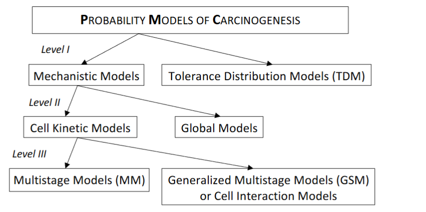
Figure 4.1: A classification of the stochastic models of carcinogenesis.

The compact presentation and discrimination in Figure 4.1 has been taken place at first level according to the intention, at second level according to biological detail and at third level according to the desired method, and is based on the above discussion.

5. Theoretical Implications in Practice

There is a need for calculating low level percentiles, Kitsos,⁵³ working for low dose extrapolation problems. For practical reasons the calculation should be simple such that it can be adopted easily be the experimentalist, while at the same time, this derivation has to be optimal in the statistical sense. One of the targets of this paper has been to refer on the calculation of the low-dose percentiles by adopting the sequential principle of design, Hu.⁵⁴ The sequential approach can be faced easier through the stochastic approximation scheme. This is discussed below in comparison with a static design approach: i.e., perform once an experiment.

Example 5.1 Recall the One Hit model F(x)=1−exp⁡(−θx),θ>0,x≥0F(x) = 1 – \exp(-\theta x), \theta > 0, x \geq 0F(x)=1−exp(−θx),θ>0,x≥0.

According to the definition of the percentile point it is F(Lp)=1−exp⁡(−θLp)=p⇒Lp=(−1θln⁡(1−p))1/k(5.1)F(L_p) = 1 – \exp(-\theta L_p) = p \Rightarrow L_p = \left(-\frac{1}{\theta} \ln(1 – p)\right)^{1/k} \quad (5.1)F(Lp)=1−exp(−θLp)=p⇒Lp=(−θ1ln(1−p))1/k(5.1)

This result can be generalized. It has been proved, Kitsos,⁵⁵ that within the class of Multistage Models there exists an iterative scheme which converges to the percentile LpL_pLp. Such a need is essential when ppp is very small and can always be evaluated sequentially, rather than working with a static design, as the estimated percentile is re-estimated.⁵⁶

Another point of interest, with a strong theoretical background, is mixtures. Humans are exposed to a large number of chemicals from a variety of different sources, either sequentially or static/concurrently. We would like to clarify that mixtures of chemicals are ubiquitous:

in the air the animals and humans are breathing
the food that all species are eating
the water that all species and especially humans are drinking

Therefore, an extended analysis to the involved chemical mixtures is needed to provide a further analysis on Cancer Risk Assessment, Kitsos and Edler,⁵⁷ who worked on the different Statistical models concerning the mixtures and the corresponding Geometrical presentation, to clarify the situation to the experimenter.

A simple chemical mixture consists of a composition of chemicals. In practice this composition consists of no more than ten chemicals. The qualitatively and quantitatively synthesis is supposed to be known, in any case, that means that even if it is not known has to be investigated and analysed. The various combination of chemicals can eventually affect on either different target organs or the same target organ.

The above two groups can be combined with the two assumptions on the action of these chemicals. This action is consisted of chemicals that can be either with different mode of action or with the same mode of action.

The main terms in a biological mixture bioassay, when a mixture experimental approach is adopted for the biological/toxicological problem, under investigation, has been developed by Hodgson and Levi,⁵⁸ Kitsos and Edler⁵⁷:

Synergism: Both involve toxicity greater than would be expected from the toxicities of the compounds administrated separately, by the case of synergism one compound has little or no intrinsic toxicity administrated alone, where in the case of
Potentiation: both compounds have appreciable toxicity when administrated alone.

As a toxicological interaction, the National Research Council (NRC),²⁰ defines a circumstance in which exposure to two or more chemicals results in a qualitatively or quantitatively altered biological response relative to that predicted from the actions of a single chemical.log⁡(p(x)1−p(x))=xT=β0+β1×1+⋯+βpxp,\log\left(\frac{p(x)}{1 – p(x)}\right) = x^T = \beta_0 + \beta_1 x_1 + \cdots + \beta_p x_p,log(1−p(x)p(x))=xT=β0+β1x1+⋯+βpxp,

Hosmer and Lemeshow,⁶¹ Rao and Toutenburg,⁶² we can evaluate thatp(x)=Logit−1(xTβ)p(x) = \text{Logit}^{-1}(x^T \beta)p(x)=Logit−1(xTβ)

which remains invariant under affine transformations,⁶⁶ while for a development of the Generalized Linear Models see Collett,⁶⁷ Cox and Snell.²⁷ A very similar approach had been adopted by Bliss⁶⁸ in his pioneering paper of Risk Analysis, were counting the number of dead insects after being exposed to CS2CS_2CS2.

Usually, interest is focused on the Relative Risk (RR), with RR=exp⁡(β1)RR = \exp(\beta_1)RR=exp(β1) and we test the null hypothesis H0:RR=1H_0: RR = 1H0:RR=1 vs the alternative H1:RR≠1H_1: RR \neq 1H1:RR=1. The Chi-square test, Lemeshow and Hosmer⁶⁹ among others, is very useful, when a “large” number of observations are considered, while the hazard function has been also proved useful to the experimenter, especially when the time is part of the whole study. Although the Normal distribution has been generalized and the hazard function for the Generalized Normal has been evaluated, Toulias and Kitsos,⁷⁰ the researcher still needs the classic hazard function, as it is easier to be evaluated and there are not Mathematics associated with it.

Example 5.2. Some of the markers related to the breast cancer are widely monitored and the relevant tests are routinely performed on patient samples, with the following being the most popular: Estrogen Receptors (ER), Progesterone Receptors (PR), HER-2, p53, S phase. Many gene polymorphisms in the metabolism of breast cancer have been described as possible neoplasm etiologic factors, Bugano et al.⁷¹ Regarding the breast cancer risk assessment, susceptibility, and its relation to CYP17, MspA1 polymorphism, different opinions have been expressed, Feigelson et al.,⁷² while Huang et al.⁷³ found a positive association between the breast cancer relative risk and the individual susceptibility genotypes. See Kitsos⁷⁴ for the details of this study, while the method was extended for the Generalized Normal distribution and Information criteria providing an appropriate software, Kitsos and Toulias.⁷⁵

Therefore, a study was performed referring to 98 breast cancer patients and 125 healthy controls where they were compared considering the age at menarche, age at menopause, the number of full-term pregnancies and the CYP17, COMT genotypes. The frequency of CYP17 A1/A1 genotype was compared to A1/A2 and A2/A2, whereas the frequency of COMT G/G genotype was compared to G/A and A/A. The result was that the full pregnancy with Relative Risk, RR=1.42RR = 1.42RR=1.42 and Menopause with RR=1.04RR = 1.04RR=1.04 (p<0.05p < 0.05p<0.05) influence the final RR.

Interpretation of the coefficients of the statistically significant variables, provide evidence, that on the basis of this study, when the age at menopause increases one year the probability of breast cancer increases 4%.

Moreover, women with full time pregnancy have 42% less probability for breast cancer than other women. In that point it is useful to remark that from the interpretation of the coefficient of the variable age of menarche from the full model we have that when the age of menarche increases one year then the probability of cancer decreases 5%. There is a strong interest on the subject from the statistical point of view, see Duffy,⁷⁶ Prentice and Gloeckler,⁷⁷ among others.

6. Conclusion

It has mentioned that tumour markers (usually proteins associated with a malignancy) might be clinically usable in patients with cancer, Cheung et al.,⁷⁸ Amaral-Mendes and Pluygers.⁷⁹ A tumour marker can be detected in a solid tumour, in circulating tumour cells in peripheral blood, in lymph nodes, in bone marrow or in other body fluids. As the problem of Carcinogenesis is so important a number of models have been already reviewed, Vineis et al.,⁸⁰ while others provide new ones, Gatenby and Vincent,⁸¹ as it is expected due to the evolution.

The aim of this paper has been to offer Statistical methods and discussion either for experimental carcinogenesis problems or for real life Cancer problems. The former needs extrapolation to humans or interspecies extrapolation, Travis et al.,⁹ while the latter is a real problem with the most references in the Science, Edler and Kitsos,¹⁰ Crump et al.⁸³ Different accidents, the main one being the Chernobyl, Baverstock and Williams,⁸⁴ among others, provided less information than it was expected, due to the problems to collect the appropriate data. As the Risk Assessment of Cancer has studied in detail from the medical, Ladenson,⁸⁵ Kawai et al.,⁸⁶ Hayat et al.,⁸⁷ toxicological studies, Bowman et al.,⁸⁸ and biological points of view, Arden et al.,⁸⁹ the main objective of this work has been to provide an insight into this problem from the Statistical point of view proposing a sequential bioassay for the estimation of low-dose exposure, i.e. low-dose percentiles.

The optimal experiment design has been adopted and the sequential principle has been considered. Static designs, where all the observations are used once have the disadvantage that a costly experiment might be performed and the acquired estimator might be far from the “true” value. The effect of covariates in Cancer problems, it is always a useful idea to proceed, Petersen,⁹⁰ Kitsos.⁴⁰

The Probability Models it is not related to epidemiological studies, Fley et al.,⁹¹ Horn-Ross et al.,⁹² Kafadar and Tukey,⁹³ among others. These studies can be helpful in constructing statistical parameters, and being helpful in Risk Analysis studies. We strongly encourage the development and use of such models trying to explain the underlying mechanics through Statistical modeling. It is better to approach the situation with an error than to have no model to describe the phenomenon. In the development we attempted, mainly based on our research work, we believe that Luebeck et al.,³⁸ Montie and Meyers³⁹ are among those who tackled the real problem, while the majority of Statistical work offer ideas for facing the problem, as it happens to Risk Analysis which oscillates between practice and theory, Kitsos.¹⁸ But still we believe that a simple geometrical figure clarifies the situation, providing food for investigating the Statistics behind. It is a real need the Statistical coverage, usually through an appropriate, and assumed correct, model. There are a number of theoretical techniques, trying to support the research on this kind of Bioassays.

The affine Geometry approach for the invariance of the logistic model, Kitsos,⁶⁴ can be useful on defining the appropriate transportation from animals to humans (usually it is assumed the transformation: the body weight to the power around the value of 0.74), while Hermann et al.³¹ provided more Mathematics to study the surface of a tumour. Statistics is the right hand of Sciences, so we believe it can proved herself useful facing Cancer problems, communicating with Medicine and Biology. The advice “Keep It Simple”, Kitsos,²⁸ is depending on the definition of “simple”, which is a function of time. What is “simple” today was not 50 years ago, with typical examples being the conic sections of Apollonius, which were waiting for centuries Kepler to adopt them. Now ellipse, parabola etc. are simple questions at high schools. Therefore, it needs determination, and capable communication skills, to adopt the Probability models of today to study, in a team work, the evolution of the cancer problems.

Conflict of Interest:
None

Acknowledgments:
CPK would like to thank the CCMS/NATO pilot study for the generous grand, on carcinogenesis, for the time period 1990–2008 and the participants for the nice discussions. The comments of the referees are very much appreciated and help us to promote the final form of this paper.

References

1. Baish WJ, Jain KR. Fractals and Cancer. Cancer Research, 2000; 60:3683-3688.

2. Tan WY. Stochastic Models of Carcinogenesis. Marcel-Dekker, N.Y.;1991

3. Wosniok W, Kitsos C, Watanabe K. Statistical issues in the Application of Multistage and Biologically Based Models. In: Cogliano V, Luebeck G, Zapponi G. eds. Respectives on Biologically Based Cancer Risk Assessment. NATO-Challenges of Modern Society. 1998; Vol. 23:243-272.

4. Zapponni, G. A. Carcinogenetic Risk Assessment: Some Points of Interest for a Discussion. In: Chyczewski L, Niklinski J, Plugers E. eds. Endocrine Disrupters and Carcinogenic Risk Assessment. IOS press. 2002; 15-27.

5. Bernal M, Chalikias MS, Kitsos CP. Analysing data set on Thyroid Cancer. In: 2d International Conference on Cancer Risk Assessment (ICCRA2, e-proceedings). 2007; Santorini, 25-27 May 2007.

6. Hayat MJ, Howlader N, Reichman ME, Edwards BK. Cancer statistics, trends, and multiple primary cancer analyses from the Surveillance, Epidemiology, and End Results (SEER). Program Oncologist. 2007; 12:20-37.

7. Angelopoulou R, Bala M, Lavranos G, Chalikias M, Kitsos C, Baka S, Kittas C. Evaluation of immunohistochemical markers of germ cells’ proliferation. In the developing rat testis: A comparative study. Tissue and Cell. 2008; 40(1):43-50

8. Cogliano VJ, Luebeck EG, Zapponi G. Perspectives on Biologically-Based Cancer Risk Assessment eds. NATO Challenges of Modern Society. Kluwer Academic/Plenum Pub. 1999; Vol 23.

9. Chyczewski L, Niklinski J, Pluygers E. Endrocrine Disruptors and Carcinogenic Risk Assessment. NATO Science Series I. IOS Press. Amsterdam; 2002; Vol 340.

10. Edler L, Kitsos, CP. Recent Advances in Qualitative Methods in Cancer and Human Health Risk Assessment. Editors, Wiley, UK; 2005.

11. Moolgavkar SH, Venzon D. Two-Event Modls for Carcinogenesis: Incidence Cures for Childhood and Adult Tumors. Mathem. Biosciences. 1979; 47:55-77.

12. Moolgavkar SH, Knudson A. Mutation and cancer: A model for human carcinogenesis. Journal of the National Cancer Institute. 1981; 66:1037-1052.

13. Luebeck GE, Moolgavkar SH. Two-Event Model for Carcinogenesis: Biological, Mathematical and Statistical Considerations. Risk Analysis. 1989; 10:323-341.

14. Luebeck GE, Moolgavkar SH. Stochastic Description of Initiation and Promotion in Experimental Carcinogenesis. Ann. Ist. Super.Sanita. 1991; 27(4):575-580.

15. Luebeck GE, Moolgavkar SH. Multistage Carcinogenesis: Population-Based Model for Colon Cancer. Journal of National Institute. 1992; 610-618.

16. Kopp-Schneider A. Carcinogenesis models for risk assessment. Stat. Methods in Medical Research. 1997; 6:317-340.

17. Muller CH, Kitsos CP. Optimal Design Criteria Based on Tolerance Regions. In: Di Bucchianno A, Lauter H, Wynn H, eds. MODA7 – Advances in Model-Oriented Design and Analysis. Physica-Verlag. 2004; 107-115.

18. Kitsos CP. Risk Analysis in Practice and Theory. In: Kitsos CP, Oliveira TA, Pierri F, Restaino MR, eds. Statistical Modelling and Risk Analysis. Springer. 2023; 107-118.

19. Kitsos CP. Optimal Design for Bioassays in Carcinogenesis. In: Edler L, Kitsos CP, eds. Quantitative Methods for Cancer and Human Health Risk Assessment. Wiley, England. 2005; 267-279.

20. National Research Council (NCR). Principles of Toxicological Interactions Associated with Multiple Chemical Exposures. National Academic Press. Washington, DC. 1980.

21. Armitage P, Doll R. The Age Distribution of Cancer and a Multi-Stage Theory of Carcinogenesis. Brit. J. Cancer. 1954; 8:1-12.

22. Armitage P. The Assessment of Low Dose Carcinogenicity. Biometrics. 1982; 28 (sup.):119-129.

23. Armitage P. Multistage Models of Carcinogenesis. Environmental Health Perspectives. 1985; 63:195-201.

24. Doll R. The Age Distribution of Cancer: Implications for Models of Carcinogenesis. JRSS. 1971; A134:133-166.

25. Doll R. An Epidemiological Perspective on the Biology of Cancer. Cancer Res. 1978; 38:3573-3583.

26. Cox DR. Regression Models and Life Tables (with discussion). JRSS. 1972; B, 74:187-220.

27. Cox DR, Snell EJ. Analysis of binary data. Second Edition, Chapman and Hall. 1989.

28. Kitsos CP. Sir David Cox: A wise and noble statistician (1924–2022). Eur. Math. Soc. Mag. 2022; 27 – 32.

29. Stehlik M, Hermann P, Giebel S, Schenk JP. Multifractal Analysis on Cancer Risk. In: Oliveira TA, Kitsos CP, Oliveira A, Grilo L, eds. Recent Studies on Risk Analysis and Statistical Modeling. Springer. 2018; 17-34.

30. Losa GA, Nonnenmacher TF. Fractals in biology and medicine. Springer. 2005.

31. Hermann P, Piza S, Ruderstorfer S, Spreitzer S, Stehlik M. Fractal Case Study for Mammary Cancer: Analysis of Interobserver Variability. In: Kitsos CP, Oliveira TA, Rigas A, Gulati S, eds. Theory and Practice of Risk Assessment. Springer. 2015; 21-36.

32. US EPA. Guidelines for exposure assessment. Federal Register. 1992; 51:33992-34003.

33. US EPA. Guidelines for Carcinogenic Risk Assessment. EPA, Washington, DC. 1999.

34. Wosniok W, Kitsos CP, Watanabe K. Statistical issues in the Application of Multistage and Biologically Based Models. In: Cogliano V, Luebeck G, Zapponi G. Respectives on Biologically Based Cancer Risk Assessment. NATO-Challenges of Modern Society. 1998; Vol. 23:243-272.

35. Iverson S, Arley N. On the mechanism of experimental carcinogenesis. 1950; 27:773-803.

36. Nordling CO. A new theory of the cancer inducing mechanism. British J. of Ca. 1953; 7:78-72.

37. McCullagh P, Nelder JA. Generalized Linear Models. Chapman and Hall, London. 1989.

38. Luebeck EG, Watanabe K, Travis C. Biologically based models of carcinogenesis. In: Cogliano VJ, Luebeck EG, Zapponi GA, eds. Prospectives on Biologically Based Cancer Risk Assessment. Kluwer Academic/Plenum Publishers. New York. 1999; 205-241.

39. Hartley HO, Sielken RL. Estimation of ‘Safe Dose’ in Carcinogenic Experiments. Biometrics. 1977; 33:1-30.

40. Finney DJ. Probit Analysis, 3d ed. Cambridge Un. Press. 1971.

41. Dewanji A, Venzon DJ, Moolgavkar SH. A stochastic two-stage model for cancer risk assessment: II. The number and size of premaligmant clones. Risk Analysis. 1989; 9:179-187.

42. Kitsos CP, Limakopoulou A. Optimal Risk Assessment for Estimating the VSD in Experimental Carcinogenesis. In: A. Hasman et al., eds. Medical Infobank for Europe. IOS Press. 2000; 763 – 766.

43. Kitsos CP. Cancer Bioassays: A Statistical Approach. Lampert. 2012.

44. Michaelis L, Menten ML. Kinetics for Intertase action. Biochemische Zeiturg. 1913; 49:333-369.

45. Endrenyi L, Chan FY. Optimal Design of Experiments for the Estimation of Precise Hyperbolic Kinetic and Binding Parameters. J. Theor. Biol. 1981; 90:241-263.

46. Currie DJ. Estimating Michaelis-Menten Parameters: Bias, Variance and Experimental design. Biometrics. 1982; 38:907-919.

47. Gilberg F, Urfer W, Elder L. Heteroscedastic Nonlinear Regression Models with Random Effects and their Application to Enzyme Kinetic Data. Biometrical Journal. 1999; 41:543-557.

48. Toulias TL., Kitsos CP. Fitting the Michaelis-Menten Model. Journal of Comp. and Appl. Math. 2016; 296:303-319.

49. Bates DM, Watts DG. Nonlinear-Regression Analysis and its Applications. Oliver and Boyd, Edinburgh. 1998.

50. Kitsos CP. Design aspects for the Michaelis – Menten Model. Biometrical Letters. 2001; 38:53-66.

51. Kitsos CP. The Cancer Risk Assessment as an Experimental Design. In: Chyczewski L, Niklinski J, Pluygers E, eds. Endocrine Disrupters and Carcinogenic Risk Assessment. IOS Press. 2002; 37:329-337.

52. Risch A, Dally H, Edler L. Genetic Polymorphisms in Metabolising Enzymes as Lung Cancer Risk Factors. In: Edler L, Kitsos CP, eds. Recent Advances in Quantitative Methods in Cancer and Human Risk Assessment. Wiley, UK. 2005.

53. Kitsos CP. Optimal Designs for Estimating the Percentiles of the Risk in Multistage Models in Carcinogenesis. Biometrical Journal. 1999; 41, No 1:33-43.

54. Hu I. On sequential designs in nonlinear problems. Biometrika. 1998; 85:496-503.

55. Kitsos CP. Optimal Designs for Percentiles at Multistage Models in Carcinogenesis. Biometrical Journal. 1997; 41, No 1:33-43.

56. Kitsos CP. Sequential Approaches for Ca Tolerance Models. Biometrie und Medizinische Informatik Greifswalder Seminarberichte. 2011; Heft 18:87-98.

57. Kitsos CP, Edler L. Cancer Risk assessment mixtures. In: Edler L, Kitsos CP, eds. Quantitative Methods for Cancer and Human Health Risk Assessment. Wiley, England. 2005; 283-298.

58. Hodgson E, Levi EP. A textbook of modern toxicology. Elsevier, New York. 1987.

59. Prentice RL, Kalbfleisch JD. Hazard Rate Models with Covariates. Biometrics. 1979; 25-39.

60. Kitsos CP. The Role of Covariates in Experimental Carcinogenesis. Biometrical Letters. 1998; Vol. 35, No 2:95-106.

61. Begg MD, Legakos S. Loss in efficiency caused by omitting covariates and misspecifying exposure in logistic regression models. JASA. 1993; 88:166-170.

62. Berkson J. Maximum Likelihood and Minimum X2 estimates of the logistic function. JASA. 1955; 50:130-162.

63. Breslow ΝΕ, Day ΝΕ. Statistical Methods on Cancer-Research. IARC. Lyon, France. 1980; No 32.

64. Hosmer DW, Lemeshow S. Applied Logistic Regression. John Wiley. 1989.

65. Rao CR, Toutenburg H. Linear Models, 2nd ed. Springer-Verlag, N. Y. 1999.

66. Kitsos CP. On the Logit Methods for Ca Problems. In: Vonta F, ed. Statistical Methods for Biomedical and Technical Systems. Limassol, Cyprus. 2006; 335-340

67. Collet D. Modelling Binary Data. Chapman and Hall/CRC. 1999.

68. Bliss CI. The calculation of the dosage mortality curve. Annals of Applied Biology. 1935; 22:134.

69. Lemeshow S, Hosmer DW. The use of goodness-of fit statistics in the development of logistic regression models. American Journal of Epidemiology. 1982; 115:92-106.

70. Toulias TL, Kitsos CP. Hazard Rate and Future Lifetime for the Generalized Normal Distribution. In: Oliveira TA, Kitsos CP, Oliveira A, Grilo L, eds. Recent Studies on Risk Analysis and Statistical Modeling. Springer. 2018; 165-180.

71. Bugano DD, Conforti-Froes N, Yamaguchi NH, Baracat EC. Genetic polymorphisms, the metabolism of oestrogens and breast cancer: A review. European Journal Gynaecological Oncology. 2008; 29(4):313-20.

72. Feigelson SH, McKean-Cowdlin R, Henderson EB. Concerning the CYP MspA1 and breast cancer risk: a meta-analysis. Mutagenesis. 2002; 17:445-446.

73. Huang CS, Chern HD, Chang KJ, Cheng CW, Hsu SM, Shen CY. Breast Cancer Risk Associated with Genotype Polymorphism of the Oestrogen-metabolizing CYP17, CYP1A1 and COMT: A Multigenic Study on Cancer Susceptibility. Cancer Research. 1999; 59:4870-4875.

74. Kitsos CP. Estimating the Relative Risk for the Breast Cancer. Biometrical Letters. 2010; Vol 47(2):133-146.

75. Kitsos CP, Toulias TL. Generalized Information Criteria for the Best Logit Model. In: Kitsos CP, Oliveira TA, Rigas A, Gulati S, eds. Theory and Practice of Risk Assessment. Springer. 2015; 3-20.

76. Duffy MJ. CA 15-3 and related mucins as circulating markers in breast cancer. Ann Clin Biochem. 1999; 36:579–86.

77. Prentice RL, Gloeckler LA. Regression analysis of grouped survival data with application to breast cancer data. Biometrics. 1978; 34:56-67.

78. Cheung K, Graves CRL, Robertson JFR. Tumour marker measurements in the diagnosis and monitoring of breast cancer. Cancer Treat Review. 2000; 26:91–102.

79. Amaral-Mendes JJ, Pluygers E. Use of Biochemical and Molecular Biomarkers for Cancer Risk Assessment in Humans. In: Cogliano V, Luebeck G, Zapponi G. Respectives on Biologically Based Cancer Risk Assessment. NATO-Challenges of Modern Society. 1999; Vol. 23:81-152.

80. Vineis P, Schatzkin A, Potter JD. Models of carcinogenesis: an overview. Carcinogenesis. 2010; 31(10):1703–1709.

81. Gatenby AR, Vincent LT. An Evolutionary Model of Carcinogenesis. Cancer Research. 2003; 63:6212– 6220.

82. Travis CC, White RK, Ward RC. Interspecies Extrapolation of Pharmacokinetics. J. Theor. Biol. 1990; 42:285-304.

83. Crump KS, Guess HA, Deal KL. Confidence Intervals and Tests of Hypotheses Concerning Dose Response Relations Inferred from Animal Carcinogenicity Data. Biometrics. 1977; 33:437-451.

84. Baverstock K, Williams D. The Chernobyl accident 20 years on: an assessment of the health consequences and the international response. Environ Health Perspect. 2006; 114(9):1312-1317.

85. Ladenson PW. Optimal laboratory testing for diagnosis and monitoring of thyroid nodules, goiter, and thyroid cancer. Clinical chemistry. 1996; 42(1):183-187.

86. Kawai R, Mathew D, Tanaka C, Rowland M. Physiologically based pharmacokinetics of cyclosporine A: extension to tissue distribution kinetics in rats and scale-up to human. Journal of Pharmacology and Experimental Therapeutics. 1998; 287(2):457-468.

87. Bowman D, Chen JJ, George EO. Estimating Variance Function in Developmental Toxicity Studies. Biometrics. 1995; 51:1523-1528.

88. Arden KC, Anderson MJ, Finckenstein FG, Czekay S, Cavenee WK. Detection of the t(2:13) chromosomal translocation in alveolar rhabdomyosarcomah using the reverse transcriptase polymerase chain reaction. Genes Chrom Cancer. 1996; 16:254-260.

89. Petersen T. Fitting Parametric Survival Models with Time-Dependent Covariates. Appl. Statist. 1986; 35:281-288.

90. Ferlay J, Autier P, Boniol M, Heanue M, Colombet M, Boyle P. Estimates of the cancer incidence and mortality in Europe in 2006. Annals of Oncology. 2007; 18:581-592.

91. Horn-Ross PL, Morris JS, Lee M. Iodine and thyroid cancer risk among women in a multiethnic population: the Bay Area Thyroid Cancer Study. Cancer Epidemiol Biomarkers Prev. 2001; 10:979-85.

92. Kafadar K, Tukey JW. U.S. Cancer Death Rates: A Simple Adjustment for Urbanization. International Statistical Review. 1993; 61:257-281.

93. Montie JE, Meyers SE. Defining the ideal tumor marker for prostate cancer. Urol Clin North Am. 1997; 24:247-252.

Interested in publishing your own research?

ESMED members can publish their research for free in our peer-reviewed journal.

Learn About Membership