The Testing of Epidemiological Concepts during the COVID-19 Pandemic

Dr. Mauricio Canals L.^1,2

1. Programa de Salud Ambiental, Escuela de Salud Pública, Facultad de Medicina, Universidad de Chile.
2.  Departamento de Medicina, Facultad de Medicina, Universidad de Chile.

http://orcid.org/0000-0001-5256-4439

OPEN ACCESS

PUBLISHED: 30 April 2025

CITATION: Canals, M. L. (2025). The testing of epidemiological concepts during the COVID-19 pandemic. Medical Research Archives, [online] 13(4). https://doi.org/10.18103/mra.v13i4.6476

COPYRIGHT: This is an open-access article distributed under the terms of the Creative Commons Attribution License, which permits unrestricted use, distribution, and reproduction in any medium, provided the original author and source are credited.

DOI https://doi.org/10.18103/mra.v13i4.6476

ISSN 2375-1924

ABSTRACT

The COVID-19 pandemic had a profound global impact, marked by high morbidity and mortality rates. It also placed substantial strain on epidemiological understanding, complicating efforts to measure the pandemic’s scale and speed of transmission, as well as the implementation of mitigation and control strategies. Throughout the pandemic, key epidemiological concepts—such as the basic reproductive number, serial interval, incidence rate, fatality rate, and effective reproductive number—came under intense scrutiny. New concepts, like incidence moments, were even developed to better assess the scale of the outbreak and support temporal forecasting.

In this analysis, we trace the chronological relationship between the progression of the pandemic and the application of these key epidemiological concepts. We briefly examine their historical development, definitions, significance, interconnections, and how they informed both non-pharmaceutical interventions and, later, pharmaceutical measures with the introduction of vaccines. We show that the reproductive number proved to be a particularly valuable tool, guiding the design of epidemiological interventions and helping to define conditions for herd immunity and the vaccination threshold. In contrast, crude case fatality rates were often misleading, requiring adjustments to account for the time lag between infection and death. While incidence rates and reproductive numbers were essential for understanding disease burden and transmission dynamics, they were insufficient in forecasting future case counts. The concept of herd immunity was also critical, but its implications were frequently misunderstood. It was necessary to clarify that reaching the herd immunity threshold does not abruptly end an epidemic, and to highlight its dependence on vaccination thresholds and vaccine effectiveness.

Keywords

COVID-19, epidemiology, reproductive number, herd immunity, vaccination, incidence rate

Introduction

Since 2019, the COVID-19 pandemic has had a significant impact on global populations, resulting in more than 778 million cases and over 7 million deaths. Officially originating in Wuhan, China, on November 17, 2019, the virus first spread to Europe and then to the rest of the world, with the World Health Organization declaring it a pandemic on March 13, 2020. Countries worldwide adopted various strategies to address the pandemic. For instance, South Korea, China, Japan, Taiwan, and Hong Kong implemented early public health interventions, drawing from their previous experiences with SARS in 2002–2003.

China responded with early border closures, strict travel restrictions, building sanitization, extensive testing, and a significant increase in healthcare capacity. South Korea adopted an aggressive mass screening strategy, testing symptomatic individuals, contacts of confirmed cases, and travelers, while also closing schools and recommending remote work. Meanwhile, Hong Kong, Singapore, and Japan used active surveillance systems to identify cases and their contacts, developed diagnostic tests, and expanded laboratory capacity. Germany focused on testing symptomatic groups, implementing moderate contact tracing, quarantines, and isolating symptomatic individuals, while the United Kingdom emphasized strict traceability. In contrast, the United States limited testing to specific symptomatic groups and set up public testing services without enforcing strict isolation or quarantine measures in 2020 and 2021. Australia and New Zealand implemented early public health measures, including effective communication, social distancing, personal hygiene protocols, and expanded healthcare coverage.

In response to the pandemic, global efforts were made to develop COVID-19 vaccines, and by the end of 2020, three vaccines had been authorized as safe and effective by the WHO. Starting in December 2020, agreements with manufacturers were reached, emergency use authorizations were granted, and vaccines began to be administered on a large scale, initially prioritizing those at higher risk of severe illness or death, in line with ethical principles of justice and equity, as well as economic considerations. By June 30, 2022, global vaccination coverage reached 66.9% of the population with at least one dose, though only 19.6% of people in low-income countries had received at least one dose. As vaccination campaigns progressed, countries continued to confront the pandemic by combining vaccination strategies with non-pharmacological interventions. For example, Europe considered two approaches: one focused on rapidly lifting restrictions, assuming that natural exposure and vaccination would help achieve herd immunity and prevent overwhelming healthcare systems; the other aimed to gradually ease restrictions based on vaccination progress, while maintaining low case numbers and supporting an efficient test-trace-isolate (TTI) system.

As the pandemic progressed, the SARS-CoV-2 virus evolved, generating various lineages, variants, and sub-variants beyond the original strain. Chronologically, these include: α (B.1.1.7 and Q), β (B.1.35 and its descendants), γ (P.1 and descendants), δ (B.1.617.2 and descendants), ε (B.1.43), η (B.1.52), ι (B.1.53), κ (B.1.617.1), Omicron (B.1.1.529 and descendants), ζ (P.2), and µ (B.1.621 and B.1.621.1), with recombinant Omicron variants now being the most prevalent.

During the course of the pandemic, numerous questions and management challenges emerged, prompting a reevaluation of various epidemiological concepts. Initially, these inquiries focused on the virus’s origin, its reservoir, and the reservoir that facilitated its amplification. However, as the disease spread within the population, the focus shifted toward the scale and management of the pandemic.

The objective of this analysis is to establish the chronological relationship between the progression of the pandemic and the application of key epidemiological concepts. We briefly examine their historical development, definitions, significance, interconnections, and how they informed both non-pharmaceutical interventions and, later, pharmaceutical measures with the introduction of vaccines, during the COVID-19 pandemic.

At the onset of the pandemic, the primary questions that arose were about the transmissibility of the new virus and its fatality rate. In response, various studies first turned their attention to the concept of the basic reproductive number (R0).

Basic reproductive number (R0)

The concept of R0 originated in demography. The first approximation of this concept can be traced back to Richard Bockh in 1886, who, using life tables from the 1879 Berlin population, calculated what he called “die totale Fortpflanzung der Bevölkerung” (the total reproduction of the population). Bockh arrived at a value of 1.06, which may be considered the first estimate of R0 for a population. Today, in human demography, R0 is defined as the average number of daughters produced by each woman in a given generation.

The concept was defined in its current form by Alfred Lotka in 1925, who referred to it as “net fertility.” However, he had been developing the idea based on a series of works dating back to 1907. In 1911, he first introduced it in writing:

0 ( ) ( ) 1
0 > ⇔ > ∫ ∞
r b a p a da

here, b(a) represents the birth rate per individual at age “a,” and p(a) denotes the probability of survival at that age. He referred to “r” as the “per capita rate of natural increase” (or intrinsic rate of increase).

In epidemiology, the first approximation of this concept can be traced to the work of En’ko (1889), who had a clear understanding of the population threshold for the transmission of childhood diseases. However, a more refined approximation emerged from Ronald Ross’s work on malaria, where he identified the key factors in malaria transmission and calculated the number of new infections as the product of these factors. Ross further advanced the concept by determining the threshold number of mosquitoes below which malaria cannot persist in the population, a principle known as the “Mosquito Theorem.” In recognition of his contributions to malaria research, Ross was awarded the Nobel Prize in Medicine in 1902. Ross, and later Ross with Hilda Hudson, focused more on the concept of threshold mosquito density than on reproductive potential, without establishing a direct link to demography.

Fascinated by the work of Ross and Hudson, Lotka wrote an article titled “A Contribution to Quantitative Epidemiology,” in which he acknowledged the similarity between the reproduction of a population and the reproduction of a disease, stating:

0 ( ) ( ) 1
0 > ⇔ > ∫ ∞
z K p s c s ds

here, c(s) represents infectivity at time s, and p(s) is the probability that a newly infected individual remains infected at that time.

Later, in 1927, W.O. Kermack and A.G. McEndrick established the definitive connection between the threshold theorem (Mosquito Theorem) and R0. Subsequently, G. Macdonald (1952) defined the reproduction rate of malaria as “the number of infections distributed in a community as a direct result of the presence of an index case.” In the later half of the 20th century, Bailey (1957) compiled much of the information from mathematical models in epidemiology, while Dietz (1975) reformulated the concept. The classic works of Roy Anderson and Robert May (1979) further integrated the concept into modern epidemiological theory.

For directly transmitted infectious diseases, R0 can be deduced from compartmental models such as Susceptible-Infected-Recovered (SIR).

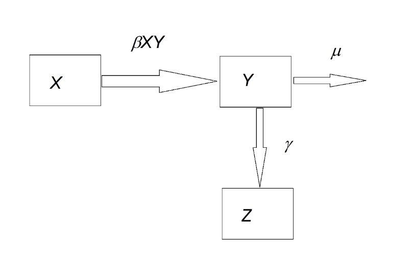
The necessary and sufficient condition for the occurrence of cases is that: dY/dt > 0. In other words, βXY – (γ + μ) > 0, which leads to βX > γ + μ and βX/(γ + μ) > 1.

By defining the reproductive number (R0) as the number of secondary cases resulting from an index case, it becomes clear that the condition for the existence of cases is R0 > 1, which is equivalent to the previous equation. In other words, we can express: R0 = βX/(γ + μ). A more formal definition of R0 is the number of secondary cases generated by a case during a generation time (its entire infectious period, T). Furthermore, if we rearrange the equation, we obtain: X > (γ + μ)/β = X*. This can be interpreted as follows: “A minimum threshold of susceptibilities (X*) is required for cases to occur.” This is referred to as the threshold theorem. Given that βX represents the reproductive potential of an infection and (1/(γ + μ)) represents the infectious life expectancy, it follows that R0 is the product of the force of infection and the infectious life expectancy.

The concept of R0 helped guide and justify epidemiological interventions during the COVID-19 pandemic. The primary epidemiological objective was to reduce R0, which can be achieved by increasing the recovery rate, γ, typically through the development of an effective treatment. However, this is not always straightforward, as observed during the pandemic. As a result, the main mitigation strategy focused on reducing the transmission coefficient (β: transmissibility). This can be broken down as: β = bP(I/C)P(C), where b is the contact rate between individuals, P(C) is the probability of infectious contact, and P(I/C) is the probability that an infectious contact leads to an infection. In the case of COVID-19, epidemiological interventions targeted one or more of these three factors:

• P(I/C): use of masks, personal hygiene measures, disinfectants such as alcohol gel, handwashing, and vaccination.
• b: mobility restrictions, disaggregation, and social distancing.
• P(C): contact tracing and isolation of infected individuals and their contacts, school and university closures, quarantines, sanitary cordons, and border closures.

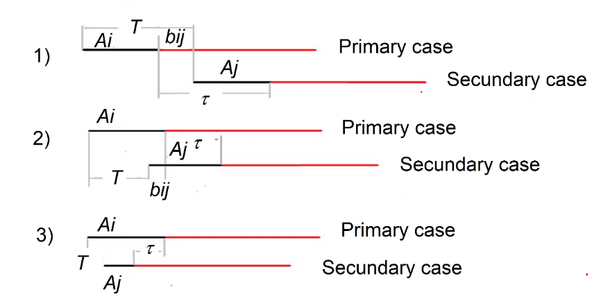
Estimating R0 is challenging because some of its parameters are influenced by the characteristics of the pathogen. The objective is to calculate R0, if possible, under the assumption that the entire population is susceptible and that no mitigation or control measures have been implemented—essentially, at the onset of an epidemic. At this stage, the epidemic curve, before any disruption caused by human intervention, reflects the uncontrolled spread of the infection within the population. A useful estimator is based on the initial quasi-exponential increase in incidence, which enables the following approximation: dI/dt = r0t ⇒ lnI = r0t + c, where I is the number of new infections, r₀ is the intrinsic rate of increase of the infection, and c is a constant. By performing a regression analysis between ln I and time t, it is possible to determine the intrinsic growth rate, represented by the slope of the regression line. This rate, r₀, is related to R0, but it is model-dependent. In its simplest form, when infectivity is constant, R0 = 1 + rτ, where τ is the serial interval, defined as the average time between the acquisition and transmission of symptomatic disease. However, this calculation can be challenging due to stochastic fluctuations, the rarity of cases, and poor case registration at the onset of epidemics. In the case of superinfectors—individuals capable of infecting a large number of others in a single event (such as when someone sneezes on a crowded subway during peak hours)—a useful approximation is: R0 = 1 + rτ + f(1 − f)(rτ), where f is the ratio between the infectious period and the serial interval. As we can see, the concept of the serial interval is crucial. Generation time (T) is defined as the average time between infections, and, as the term suggests, it is equivalent to the time between generations in population dynamics. The challenge with infectious diseases is that it is highly unlikely to pinpoint the exact moment when an infection is acquired. However, the time at which an individual becomes symptomatic can be observed. Therefore, the serial interval is defined as the average time between the acquisition and transmission of symptomatic disease. If the latent and incubation periods were constant, they would be equal; however, this is not always the case.

At the start of the pandemic, numerous studies attempted to estimate R0. A meta-analysis based on 42 studies reported an average R0 of 2.87, with a 95% confidence interval (CI): (2.39–3.44). As the pandemic progressed and new variants emerged, this value was recalculated for each variant, revealing an increase in transmission alongside a decrease in virulence. Specifically, for the α variant, R0 was reported as 3.9, with a 95% CI: (3.4–4.4); for the γ variant, R0 was 4.2, with a 95% CI: (3.5–5); for the δ variant, R0 was 5.2, with a 95% CI: (3.2–8); and for the Ο variant, R0 was 9.5, with a 95% CI: (5.5–24).

Case fatality rate (CFR)

The Case Fatality Rate (CFR) is a measure of disease severity within a population. Conceptually, it refers to the proportion of deaths caused by a disease. In its simplest form, CFR is the ratio of the cumulative number of deaths from a disease over a specific period of time (Dt) to the cumulative number of cases of that disease during the same period (Ct).

CFR = Dt/Ct = ∑ dt_i=0 / ∑ ct_i=0, where Dt and Ct represent the number of deaths and cases on day t. The number of infected individuals at the same time can also be used in the denominator, in which case it is referred to as the Infection Fatality Rate (IFR). However, estimating the IFR can be challenging, as it may be biased upward if cases are underreported, and biased downward if the delay between illness and death is not accounted for. This delay is a critical factor, as the deaths attributed to a disease at time t are the result of the sick population at an earlier time, rather than the entire sick population since the start of the epidemic. Moreover, this earlier time is a random variable with an fj distribution (i.e., the conditional probability of dying at time j given that one is sick). To address this, Nishiura et al. (2009) proposed an unbiased estimator that corrects for the delay: cCFR = CFR/u(t) where u(t) = ∑ ∑ ci−jfj_j=0 / ∑ ci_i=0. You can see that cCFR = ∑ dt_t=0 / ∑ ∑ ci−jfj_j=0.

A notable study during the pandemic involved estimating the case fatality ratio for COVID-19 using age-adjusted data from the outbreak aboard the Diamond Princess cruise ship in February 2020. In this study, the authors estimated the case fatality ratio (cCFR) on the Diamond Princess to be 2.6%, with a 95% confidence interval (CI): (0.89–6.7). By comparing deaths on board with expected deaths based on CFR estimates from China, they estimated the cCFR in China to be 1.2%, with a 95% CI: (0.3–2.7). In Chile, a study conducted from 2020 to 2023 using Lt observed a decrease in COVID-19 lethality, from values close to 4% with the original variant, α, and γ, to values around 1% with the O variant.

Incidence rate

The daily incidence rate is a valuable parameter for monitoring cases of an infectious disease like COVID-19. It is expressed as the ratio of the number of new cases (Ct) on a given day to the exposed population (Pt) at that time:

It = ct/Pt (unit of time).

Typically, in rapid processes, the population remains constant. When characterizing a specific locality, the population can be omitted and the metric can simply be referred to as cases per day. However, when comparing different populations, it is essential to include Pt. The incidence rate serves both as a measure of the disease burden in the population over a given period and as an indicator of the speed at which the disease spreads. Once the epidemic was established, the incidence rate, along with the CFR, became the most commonly used parameters to describe the COVID-19 pandemic.

Effective reproduction number

The incidence rate alone is insufficient to measure disease transmission. While it provides information about the number of cases over time, it offers no insight into the transmission process, i.e., the origin of the cases. The concept of the effective reproductive number (Rt) refers to the number of secondary cases generated from a single case during the course of the disease’s progression in the population. Like R0, if its value is greater than one, the epidemic is expanding; if it is less than one, the epidemic is declining. Although it is based on the same principles and parameters as R0, Rt differs in that it takes into account factors such as the fraction of susceptible individuals (qt). This is because, during the course of an epidemic, the proportion of susceptibles is less than 1. Therefore, only qt susceptibles will be able to generate new cases, while p = 1 – qt will not. Thus, we have:

Rt = qt * R0.

This relationship establishes the connection between R0 and the effective reproductive number, a concept that CEG Smith first proposed in 1970. However, during the transmission of an infectious disease, not only does the fraction of susceptible individuals vary, but so do factors like transmissibility (β), contact rates between individuals, recovery rates (γ) due to changes or improvements in treatments, probabilities of contagion, and viral evolution. For these reasons, a more accurate expression is:

Rt = qt * β(t) * Et,

where β(t) is the time-varying transmission coefficient, and Et is the infectious life expectancy, defined as 1 / (μ + γ), where γ is the recovery rate and μ is the mortality rate.

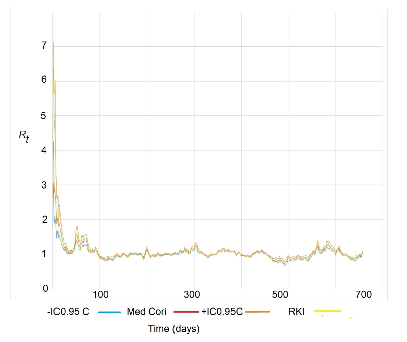
There are several methods for estimating Rt, including those proposed by Wallinga & Teunis, Wallinga & Lipsitch, Bettencourt and Ribeiro, the Robert Koch Institute (RKI), and Cori et al. In a recent review, Gostic et al. recommended the Cori approximation for real-time estimation of Rt. However, the RKI method is quick and simple to calculate, providing a point estimate for Rt based on the same principles as the Cori method. It relies on the idea that Rt can be estimated as the ratio between the current number of cases (incidence) and the cases that led to them a serial interval earlier, taking into account a variable serial interval j with a corresponding density function w(j):

Rt = It / ∑ I(t−j)w(j)_j=tj=1.

In this method, the calculation is simplified as: Rt,τ = It / I(t−τ). However, it is recommended to calculate: Rt,τ = Et / E(t−τ), as it provides more stability. In other words, it is the ratio between the moving average of the number of daily cases over the past 7 days and the moving average of the same duration, but shifted τ days earlier. For example, if τ = 5 days, it represents the ratio between the 7-day moving averages, shifted by 5 days. The Cori method, on the other hand, uses a Bayesian approximation to address the problem. It assumes that the number of infected individuals follows a Poisson distribution and that Rt = It / ∫ I(t−T)w(T)dT.

The latter expression is the same as the one above but for continuous It, with the exception that Cori uses the generation time T instead of τ. Cori applies a Gamma distribution for Rt, and since a Poisson distribution is used for It, the posterior distribution of Rt is also a Gamma distribution. This allows for the calculation of credibility intervals for Rt. The estimates of Rt using the Cori and RKI methods were widely used during the COVID-19 pandemic, producing very similar results.

Incidence moments

The COVID-19 pandemic highlighted the limitations of many epidemiological measures in describing the spread of an epidemic. Prevalence, incidence, incidence rate, and mortality were useful descriptive concepts for measuring the burden of disease in the population. On the other hand, the effective reproductive number (Rt) served as a measure of the speed of disease spread within the population. While it is true that the reproductive number, due to its conceptual framework, provides insight into key factors for intervening to mitigate and control an epidemic, it was insufficient on its own for decision-making. To make a physical analogy: during the pandemic, we asked ourselves which was more difficult—stopping a fast-moving bicycle (low mass, high speed) or a slow-moving train (high mass, low speed)?

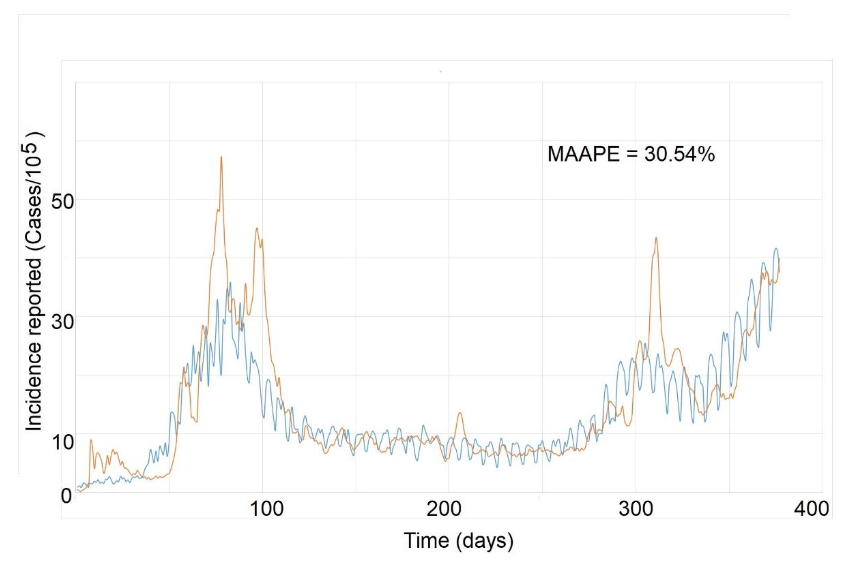
During the pandemic, the concept of “Incidence Moments” was proposed as a way to measure the “memory” of an epidemic and predict its course. The Imn = IRn is defined as the nth moment of incidence, where I represents the 7-day moving average of the incidence (I = (It + It−1 + … + It−6)/7). Thus, the first moment of incidence (or simply momentum = Im₁) is the incidence rate (IRt), which is a joint measure of both the load and speed of an epidemic. Since Rt measures the number of new cases produced by each case in a generational time (T, the average time between infection and subsequent infection), it is also a predictor of the expected incidence over a generational time T. As this time is difficult to measure during an epidemic, it is typically replaced by the serial interval (τ). We proposed that the nth moment of incidence could predict the incidence reported after “nτ” days. For example, the second moment of incidence (Im₂ = IR₂) would represent the expected incidence over two serial intervals (2τ, or approximately 10 days for COVID-19), assuming that the incidence and effective Rt remain constant. Therefore, while the first moment of incidence measures both the load and speed of an epidemic, higher-order moments not only provide a short-term forecast of the epidemic’s incidence but also allow us to assess the “memory” of the infection dynamics when compared to observed incidences. For instance, we demonstrated that the third moment of incidence (Im₃ = IR₃) had strong predictive capacity in COVID-19 epidemic. This meant that incidence could be predicted up to 3τ (approximately 15 days), providing a critical time window for implementing mitigation and control interventions. Consequently, the concept of incidence moments seems both necessary and useful for monitoring future epidemics. It offers a way to measure, on one hand, the joint load and speed of an epidemic (momentum) and, on the other, the memory and prediction window of epidemic dynamics (Im₂, Im₃…).

Herd Immunity

As the pandemic progressed and vaccines became available, the key question was what proportion of naturally or artificially immunized individuals was required to reduce the number of cases. Population, community, or herd immunity can be defined as the proportion of individuals within a group who are immune. This concept is based on the idea that the risk of infection among susceptible individuals decreases when a significant proportion of individuals are immune, known as the “herd effect” or what J. Brownlee referred to as the dilution of susceptibles in cases. Considering the relationship Rt = qt R0, it can be proposed that the necessary condition for the incidence of cases to decrease is Rt < 1. This implies qt R0 < 1, which is equivalent to (1 – pt) R0 < 1, where pt is the proportion of immunized individuals. It also leads to the inequality pt > (1 – 1/R0). Therefore, the threshold proportion of immunized individuals (either infected or vaccinated) that makes Rt < 1 and causes the incidence of infections to decrease is given by p* = 1 – 1/R0.

It is clear that reaching this threshold does not cause the epidemic to stop abruptly; instead, it begins to decline as Rt drops below 1. Another important aspect to consider is the possibility of achieving herd immunity. One of the assumptions in SIR and SEIR models is that immunity is permanent once an individual has been infected. However, this is not always the case. If immunity is not lost, achieving herd immunity naturally becomes a matter of time. The loss of immunity, however, would impact the p* threshold value. In this scenario, reaching the threshold depends on the balance between the rate of recruitment of infected individuals and the rate at which immunity is lost. The higher the rate of immunity loss, the longer it will take to reach the p* threshold. Even once this threshold is reached, new outbreaks (epidemic recurrences) may occur due to the replenishment of susceptible individuals.

There are two key points to highlight from the results above. First, all SIR or SEIR epidemiological models are based on the assumption of a homogeneous population mix, which is rarely the case in reality. Second, if p* is considered equivalent to the vaccination threshold (Vc), the effectiveness of the vaccine (e) must be factored into the formulation. Vaccine effectiveness is defined as the reduction in transmission of the infection to and from vaccinated individuals, compared to control individuals in the same population. This is similar to conventional vaccine efficacy, but it focuses on measuring protection against transmission rather than protection against the disease itself. In this case:

Vc = (1 – 1/R0)e.

An important consideration regarding vaccines is the rate at which vaccine-induced immunity is lost. If immunity is not permanent and there is a rate of immunity loss, denoted as “ϕ,” it has been suggested that a correction factor should be taken into account in Vc:

Vc = (1 – 1/R0)e / (1/e0 + ϕ).

That is, infectious disease control through vaccines depends on R0, the effectiveness of the vaccine, and the durability of vaccine-induced immunity. The impact of population heterogeneity, however, is more complex. During the COVID-19 pandemic, once vaccines became widely available, numerous studies on herd immunity were conducted. Some models have considered interactions between different age groups, while others have used spatially explicit models parameterized with transport data. Recent studies have shown that when there is heterogeneous mixing within the population between individuals of different ages, each with different transmission rates, the threshold p* (and therefore Vc) can drop from 60% to 55.8% if R0 = 2.5. If there is heterogeneous mixing between groups with varying social activity levels and different transmission rates, the threshold p* can decrease from 60% to 46.3%. When both conditions are present, the threshold can drop further to 43%.

Another study looked at a heterogeneous population with a subgroup resistant to infection and varying levels of interaction between subpopulations. This study found that as the proportion of resistant individuals increases, the threshold p* decreases, potentially reaching as low as 30% when there is more mixing between subpopulations, particularly when resistant individuals interact with the non-resistant group. This effect can be explained by the fact that resistant individuals tend to form clusters that limit the spatial spread of the virus, creating a “dilution” effect (in the Brownlee sense) that reduces the probability of transmission. These authors suggest that, for the current epidemic, seropositivity levels of 10–20% may be fully compatible with local immunity levels approaching p*. They believe the risk and scale of resurgence may be lower than currently perceived.

In the case of COVID-19, achieving herd immunity is challenging for several reasons. On one hand, there is resistance to vaccination within certain population groups, some of which are completely unjustified, such as anti-vaccine groups, and others which are based on valid concerns, such as those of pregnant women, children, and individuals with immunosuppressive conditions. These concerns delay vaccination campaigns. On the other hand, there is the issue of the loss of vaccine-induced immunity, as well as the possibility that some variants may evade vaccine-induced immunity, which increases the risk of reinfection with SARS-CoV-2.

Conclusions

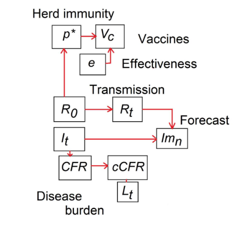
Epidemiological knowledge has been and continues to be crucial for the mitigation of the pandemic, and we have seen how all these concepts, which generally have a long history, are deeply interconnected. This meant that fully understanding one concept often required grasping another, sometimes by exploring its historical origins. For example, the thresholds for herd immunity and vaccination cannot be fully understood without understanding their relationship to Rt and R0. Many epidemiological concepts were tested successively during the pandemic. First, to estimate the virus’s transmission capacity and its lethality (R0 and cCFR). Then, to measure the disease burden on the population and health systems (It, Lt). As mitigation measures were implemented, it became important to revisit the concepts of disease burden and transmission speed (It, Rt). When necessary, new concepts were developed for short-term forecasting (Imn). As the epidemic progressed and vaccines became available, it became essential to explore the concept of herd immunity and its relationship with vaccine effectiveness and both, basic and effective reproductive number (p, Vc, R0, Rt). Perhaps the most useful concepts were R0, Rt, and, finally, herd immunity, with the latter being the most revisited today, now that vaccines are available.

References

1. World Health Organization. COVID-19 deaths dashboard. World Health Organization. https://data.who.int/dashboards/covid19/deaths?n=o. Published 2025. Accessed March 17, 2025.
2. Mizumoto K, Kagaya K, Chowell G. Transmissibility of 2019 novel coronavirus: zoonotic vs. human-to-human transmission, China, 2019-2020. medRxiv preprint. Published March 16, 2020. doi:10.1101/2020.03.16.20037036.
3. Wang J, Wang Z. Strengths, Weaknesses, Opportunities and Threats (SWOT) Analysis of China’s Prevention and Control Strategy for the COVID-19 Epidemic. Int J Environ Res Public Health. 2020; 17(7):2235. doi:10.3390/ijerph17072235.
4. Salazar Mather T, Gallo Marin B, Medina Perez G, Christophers B, Paiva ML, Oliva R et al. Love in the time of COVID-19: negligence in the Nicaraguan response. Lancet Glob Health. 2020; 8(6): E773. doi: 10.1016/S2214109X(20)301315.
5. Sebastiani G, Massa M, Riboli E. Covid–19 epidemic in Italy: evolution, projections and impact of government measures. Eur J Epidemiol. 2020; 35:341-345. doi: 10.1007/s10654-020-00631-6.
6. Peña S, Cuadrado C, Rivera-Aguirre A, Hasdell R, Nazif-Munoz J, Yusuf M et al. PoliMap: A taxonomy proposal for mapping and understanding the global policy response to COVID-19. Polimap COVID-19. 2020; [accessed 2020]. https://polimap.org/.
7. Nussbaumer‐Streit B, Mayr V, Dobrescu AI, Chapman A, Persad E, Klerings I, et al. Quarantine alone or in combination with other public health measures to control COVID-19: a rapid review. Cochrane Database Syst Rev. 2020; 15(9):9. doi:10.1002/14651858.CD013574/full.
8. WHO-Europe. Strengthening the health system response to COVID-19. Recommendations for the WHO European Region. Policy brief 2020; [accessed 2020]. http://www.euro.who.int/__data/assets/pdf_file/0003/436350/strengthening-health-system-response-COVID-19.pdf?ua=1.
9. WHO. Overview of Public Health and Social Measures in the context of COVID-19. 2020; [accessed 2020]. https://www.who.int/publications/i/item/overview-of-public-health-and-social-measures-in-the-context-of-covid-19.
10. WHO. Critical preparedness, readiness and response actions for COVID-19: Interim guidance; 2020; [accessed 2020]. https://www.who.int/publications/i/item/critical-preparedness-readiness-and-response-actions-for-covid-19.
11. Chilean Government COVID-19 Official Reports 2020; [accessed 2020]. https://www.gob.cl/coronavirus/cifrasoficiales/.
12. Cori A, Ferguson NM, Fraser C, Cauchemez S. A new framework and software to estimate time-varying reproduction numbers during epidemics. Am J Epidemiol. 2013;178(9):1505–12. doi:10.1093/aje/kwt133.
13. Nishiura H, Linton NM, Akhmetzhanov AR. Serial interval of novel coronavirus (COVID-19) infections. Int J Infect Dis. 2020; 93: 284-6. doi:10.1016/j.ijid.2020.02.060.
14. Sanche S, Lin YT, Xu C, Romero-Severson E, Hengartner N, Ke R. High Contagiousness and Rapid Spread of Severe Acute Respiratory Syndrome Coronavirus 2. Emerg Infect Dis. 2020; 26(7):1470-1477. doi:10.3201/eid2607.200282.
15. Lee VL, Chiew CJ, Khong WX. Interrupting transmission of COVID-19: lessons from containment efforts in Singapore. J Travel Med. 2020; 13:taaa039. doi:10.1093/jtm/taaa039.
16. Russell T, Hellewell J, Abbott S, Golding N, Gibbs H, Jarvis CI, et al. Using a delay-adjusted case fatality ratio to estimate under-reporting. CMMID; London School of Hygiene & Tropical Medicine; 2020. [accessed 03/2025]. CMMID Repository. https://cmmid.github.io/topics/covid19/global_cfr_estimates.html.
17. Russell TW, Hellewell J, Jarvis CI, van Zandvoort K, Abbott S, Ratnayake R, et al. Estimating the infection and case fatality ratio for coronavirus disease (COVID-19) using age-adjusted data from the outbreak on the Diamond Princess cruise ship. Euro Surveill. 2020; 25(12): 2000256. doi: 10.2807/1560-7917.ES.2020.25.12.2000256.
18. Gonzalez RI, Muñoz F, Moya PS, Kiwi M. Is a COVID19 quarantine justified in Chile or USA right now? MedRxiv 2020. [accessed 2020]. doi: 10.1101/2020.03.23.20042002.
19. Canals M. Evolución de la virulencia de SARS CoV-2 en Chile. Rev Chil Infectol. 2023; 40(6):644-650. doi: 10.4067/s0716-10182023000600650.
20. Morens DM, Breman JG, Calisher GH, Doherty PC, Hahn BH, Keush GT, et al. The origin of COVID-19 and why it matters. Am J Trop Med Hyg. 2020; 103(3): 955-959. doi: 10.4269/ajtmh.20-0849.
21. Liu Y, Gayle AA, Wilder-Smith A, Rocklöv J. The reproductive number of COVID-19 is higher compared to SARS coronavirus. J Travel Med. 2020; 27(2): taaa021. doi: 10.1093/jtm/taaa021.
22. Billah A, Miah M, Khan N. Reproductive number of coronavirus: A systematic review and meta-analysis based on global level evidence. PLoS One. 2020; 15(1): e0242128. doi:10.1371/journal.pone.0242128.
23. Böckh R. Statistiches Jahrbuch der Stat Berlin. P. Stankiewitz, 1886; Berlin.
24. Heffernan JM, Smith RJ, Wahl LM. 2015. Perspectives on the basic reproductive ratio. J. R. Soc. Interface. 2015; 2(4):281-293. doi: 10.1098/rsif.2005.0042.
25. Lotka A. Elements of physical biology. Williams & Wilkins, 1925; Baltimore.
26. Fine PEM. Ross’s a priori pathometry – a perspective. Proc Roy Soc Med. 1975; 68: 547-551.
27. Massad E, Bezerra FA. Vectorial capacity, basic reproduction number, force of infection and all that: formal notation to complete and adjust their classical concepts and equations. Mem Inst Oswaldo Cruz. 107(4): 564-567. doi: 10.1590/s0074-02762012000400022.
28. Lotka A. A contribution to quantitative epidemiology. J Wash Acad Sci. 1919; 9(3): 73-77.
29. Kermack WO, McKendrick AG. A Contribution to the Mathematical Theory of Epidemics. Proc Roy Soc Lond. A. 1927; 115: 700-721.
30. Macdonald G. The analysis of the sporozoite rate. Trop Dis Bull. 1952; 49: 569-586.
31. Bailey N. The mathematical theory of infectious diseases and its applications. Griffin 1975; London.
32. Dietz K. Transmission and control of arbovirus diseases. In Ludwig D, Cooke KL (eds) Epidemiology (.) SIAM. 1975; 104-121. Philadelphia, 1975. p. 104-21.
33. Dietz K. The incidence of infectious diseases under influence of seasonal fluctuations. Lect Notes Biomath. 1976; 11: 1-15.
34. Anderson R, May R. Population biology of infectious diseases: Part I. Nature 1979; 280: 361-367.
35. May R, Anderson RM. 1979. Population biology of infectious diseases: Part II. Nature. 1979; 280, 455-461.
36. Anderson R. Epidemiology. In: Cox FEG (ed) Modern Parasitology 1993; 75-116. Blackwell Scientific Publications, Oxford.
37. Canals M. Learning from the COVID-19 pandemic: Concepts for good decision-making. Rev Med Chile 2020;148: 415-20. https://www.scielo.cl/pdf/rmc/v148n3/0717-6163rmc-148-03-0418.pdf.
38. Canals M. Concepts for good decision-making during the COVID-19 pandemic in Chile. Point of View. Rev Chil Infectol. 2020; 37(2): 170-2. doi: 10.4067/s071610182920000200170.
39. Davies NG, Abbott S, Barnard RC, Jarvis CL, Kucharski AJ, Munday JD. Estimated transmissibility and impact of SARS-CoV-2 lineage B.1.1.7 in England. Science 2021; 372. doi: 10.1126/science.abg3055.
40. Banho CA, Sacchetto L, Campos GR, Bittar C, Possebon FS, Ullman LS, et al. Impact of SARS-CoV-2 Gamma lineage introduction and COVID-19 vaccination on the epidemiological landscape of a Brazilian city. Comm. Med. 2022; 2: 41. doi: 10.1038/s43856-022-00108-5.
41. Liu Y, Rocklöv J. The effective reproductive number of the Omicron variant of SARS-CoV-2 is several times relative to Delta. J Trav Med. 2022;1-4. doi.org/10.1093/jtm/taac037.
42. Nishiura H, Klinkenberg D, Roberts M, Heesterbeek JAP. Early epidemiological assessment of the virulence of infectious diseases: a case study of an influenza pandemic. PLoS ONE. 2009; 4(8):e6852. doi:10.1371/journal.pone.0006852.
43. Smith CEG. Prospects for the control of infectious disease. Proc Roy Soc Med. 1970; 63: 1181-90. PMID: 5530322.
44. Gostic KM, McGough L, Baskerville E, Abbott S, Joshi K, Tedijanto C, et al. Practical considerations for measuring the effective reproductive number, Rt. PLoS Comput Biol. 2020; 16(12): e1008409. doi: 10.1371/journal.pcbi.1008409.
45. Gostic KM, McGough L, Baskerville EB, Abbott S, Joshi K, Tedijanto C, et al. Correction: Practical considerations for measuring the effective reproductive number, Rt. PLoS Comput Biol. 2021; 17(12): e1009679. doi: 10.1371/journal.pcbi.1009679.
46. Wallinga J, Teunis P. Different Epidemic Curves for Severe Acute Respiratory Syndrome Reveal Similar Impacts of Control Measures. Amer J Epidemiol. 2004;160(6):509–516. doi:10.1093/aje/kwh255.
47. Wallinga J, Lipsitch M. How generation intervals shape the relationship between growth rates and reproductive numbers. Proc Biol Sci. 2007;274(1609):599–604. doi:10.1098/rspb.2006.3754.
48. Bettencourt LMA, Ribeiro RM. Real Time Bayesian Estimation of the Epidemic Potential of Emerging Infectious Diseases. PLoS ONE. 2008;3(5):e2185. doi:10.1371/journal.pone.0002185.
49. an der Heiden M, Hamouda O. Schätzung der aktuellen Entwicklung der SARS-CoV-2- Epidemie in Deutschland—Nowcasting. Epidemiologisches Bulletin. 2020;2020(17):10–15. https://edoc.rki.de/handle/176904/6650.4.
50. RKI. COVID-19 Datenhub; 2020. https://npgeo-corona-npgeo-de.hub.arcgis.com/datasets/dd4580c810204019a7b8eb3e0b329dd6_0/explore.
51. Canals M, Cuadrado C, Canals A, Johannessen K, Lefio LA, Bertoglia MP, Eguiguren P, Siches I, Iglesias V, Arteaga O. Epidemic trends, public health response and health system capacity: The Chilean experience in COVID-19 epidemic. Rev Panam Salud Publica 2020; 44, e99. doi: 10.26633/RORP.2020.99.
52. Canals M, Canals A, Cuadrado C. Incidence moments: A simple method for study the memory and short-term forecast of the COVID-19 incidence time-series. Epidemiol Meth. 2022;11(s1):20210029.doi: 10.15151/em-2021-0029.
53. Canals M, Canals A. Incidence moments: Short term forecast of the COVID-19 incidence rate in Chile. Rev Med Chile 2023; 151:823-829. doi: 10.4067/s0034-98872023000700823.
54. Fine PEM, Eames K, Heymann DL. ‘‘Herd Immunity’’: a rough guide. Clin Infect Dis. 2011; 52 (7): 911-6. doi: 10.1093/cid/cir007.
55. Fine PEM. John Brownlee and the measurement of infectiousness: an historical study in epidemic theory. J R Statist Soc A. 1979; 142 (3): 347-62. doi: 10.2307/2982487.
56. Fine P E M. Herd immunity: history, theory, practice. Epidemiol Rev. 1993; 15: 265-302. doi: 10.1093/oxfordjournals.epirev.a036121.
57. Anderson R M, May R M. Infectious diseases of humans: dynamics and control. Oxford University Press, 1991; Oxford, UK.
58. Bjørnstad BJ, Shea K, Krzywinski M, Altman N. The SEIRS models for infectious diseases dynamics. Nat Methods 2020, 17: 555-8. doi: 10.1038/s41592-020-0856-2.
59. Scherer A, McLean A. Mathematical models of vaccination. Br Med Bull 2002; 62: 187-99. doi: 10.1093/bmb/62.1.187.
60. Suryawanshi YN, Biswas DA. Herd immunity to fight against COVID-19: a narrative review. Cureus. 2023; 15(1): e33575. doi:10.7759/cureus.33575.
61. Mossong J, Hens N, Jit M, Beutels P, Auranen K, et al. Social contacts and mixing patterns relevant to the spread of infectious diseases. PLoS Med. 2008; Mar 25; 5 (3): e74. doi:10.1371/journal.pmed.0050074.
62. Colizza V, Barrat A, Barthelemy M, Vespigniani A. The role of the airline transportation network in the prediction and predictability of global epidemics. Proc Natl Acad Sci USA 2006; 2006 103 (7) 2015-2020. doi: 10.1073/pnas.0510525103.
63. Britton T, Ball F, Trapman P. A mathematical model reveals the influence of population heterogeneity on herd immunity to SARS CoV-2. Science 2020; 14; 369 (6505): 846-9. doi: 10.1126/science.abc6810.
64. Lourenço J, Pinotti F, Thompson C, Gupta S. The impact of host resistance on cumulative mortality and the threshold of herd immunity for SARS-CoV-2. 2020; doi: 10.1101/2020.07.15.20154294 doi: medRxiv.
65. Fredericksen LS, Zhang Y, Foged C, Thakur A. The long road towards COVID-19 herd immunity: vaccine platform technologies and mass immunization strategies. Front Immunol. 2020; 11: 1817. doi: 10.3389/fimmu.2020.01817.
66. Townsend JP, Hassler HB, Wang Z, Miura S, Singh J, Kumar S, Ruddle NH, Dornburg A. The durability of immunity against reinfection by SARS-CoV-2: a comparative evolutionary study, The Lancet Microbe 2 (12) (2021) e666-e675.
67. Townsend JP, Hassler HB, Sah P, Dornburg A. The durability of natural infection and vaccine-induced immunity against future infections of SARS-CoV-2. PNAS. 2022; 119 (31) e2204336119. doi:10.1073/pnas.2204336119.
68. Hirabara SM, Serdan TA, Gorjao L, Masi LN, Pithon-Curi TC, Covas DT, Curi E, Durigon EL. SARS-COV-2 variants: Differences and potential of immune evasion, Front. Cell. Infect. Microbiol. 11 (2021) 781429.
69. Angulo J, Martinez-Valdebenito C, Pardo-Roa C, Almonacid LI, Fuentes-Luppichini E, Contreras AM, Maldonado C, Le Corre N, Melo F, Medina RA, Ferrés M. Assessment of mutations associated with genomic variants of SARS-CoV-2: RT-qPCR as a rapid and abordable tool to monitoring known circulating variants in Chile, 2021, Front. Med. (Laussanne). 2022;9: 841073. doi:10.3389/fmed.2022.841073.
70. Nordström P, Ballin M, Nordström A. Risk of SARS-CoV-2 reinfection and COVID-19 hospitalization in individuals with natural and hybrid immunity: a retrospective, total population cohort study in Sweden, Lancet Infect. Dis.2022; 22 (6): 781790. doi: 10.1016/S1473-3099(22)00143-8.
71. Fine PEM. The interval between successive cases of an infectious disease. Amer J Epidemiol. 2003; 158(11): 1039-47. doi:10.1093/aje/kwg251.
72. Canals M, Canals A. Resumen analítico de la experiencia chilena de la pandemia COVID-19, 2020-2022. Cuad Méd Soc. 2022; 62(23): 7-18. doi: 10.56116/cms.v62.n3.2022.374.